- Research
- Open access
- Published:
Method of value chain mapping with international input–output data: application to the agricultural value chain in three Greater Mekong Subregion countries
Journal of Economic Structures volume 10, Article number: 6 (2021)
Abstract
Extending the technique of unit structure analysis, which was originally developed by Ozaki (J Econ 73(5):720–748, 1980), this study introduces a method of value chain mapping that uses international input–output data and reveals both the upstream and downstream transactions of goods and services, as well as primary input (value added) and final output (final demand) transactions, which emerge along the entire value chain. This method is then applied to the agricultural value chain of three Greater Mekong Subregion countries: Thailand, Vietnam, and Cambodia. The results show that the agricultural value chain has been increasingly internationalized, although there is still room to benefit from participating in global value chains, especially in a country such as Cambodia. Although there are some constraints regarding the methodology and data, the method proves useful in tracing the entire value chain.
1 Background
Participation in global value chains (GVCs) has become increasingly important as a strategy for economic development in less developed countries. Previously, industrial development proceeded in a certain order, for instance, from import to domestic production and then to the export of manufactured goods, as illustrated by the fundamental “flying geese” pattern of development (Akamatsu 1962). Simultaneously, sequences of structural transformation occur in industries, such as upgrading from (i) consumer to intermediate and capital goods and (ii) technologically simple products to complex and sophisticated ones.
However, this sequence of industrial development has become vague because of the expansion of GVCs. Indeed, a developing country can ascend into GVCs for sophisticated products, including high-tech products, by specializing in a niche segment of the value chain and becoming an exporter of these products. This phenomenon has occurred because of the rapid decline in trade and communication costs caused by technological development, trade liberalization, and regional integration. The expansion of GVCs has also affected the development strategies of developing economies. On the one hand, it is no longer necessary or efficient to build an entire value chain from scratch through infant industry protection, as assumed in Akamatsu’s (1962) model. Rather, a country can specialize in a niche segment of the value chain and then proceed to a higher value chain activity through its own upgrade efforts. On the other hand, the globalization of the economy, spurred by trade liberalization and economic integration, has narrowed the policy space for developing countries, making it increasingly difficult to protect infant industries.
Against this background, trade in value added has been explored as a method of analyzing international trade, where production processes have been increasingly fragmented across national borders and the difference between gross and value-added exports has grown rapidly.Footnote 1 In particular, VS (vertical specialization; i.e., foreign content in exports) and VS1 (domestic content used as an input for re-exports) were originally developed by Hummels et al. (2001). Subsequently, Daudin et al. (2011) presented VS1* (the domestic content of imports). Johnson and Noguera (2012) defined value-added exports. Koopman et al. (2014) synthesized these studies by tracing the value-added and double-counted elements contained in gross exports. Furthermore, Wang et al. (2017a) proposed alternative measures of GVC participation by decomposing value added and final product production in a different way and separating GVC participation into simple and complex GVC activities. Borin and Mancini (2019) proposed a different method of decompositions and developed GVC participation and vertical specialization measures that deal with double-counting terms differently.
In another methodological direction, production length and a sector’s position (i.e., relative upstreamness or downstreamness) in a value chain has been explored by economists such as Fally (2012), Antràs et al. (2012), Antràs and Chor (2013), and Miller and Temurshoev (2017). Recently, Wang et al. (2017b) developed a new set of measures for the average production length and relative upstreamness in a value chain.
However, many of these studies, which rely on the analysis of international input–output data, have focused on the structure of vertical trade particularly the acceleration of vertical fragmentation of the production process, and have not explored value chain mapping per se, which is a core element of conventional value chain analysis.
Nevertheless, value chain mapping has been conducted using different strands of research. However, the major drawback of current value chain analyses—mainly conducted by sociologists, economic geographers, and business strategists—is the lack of objective or quantitative data. For instance, a value chain map is typically drawn using information collected via interviews or other secondary sources. Consequently, “the analysis and policy recommendations provided in GVC studies are often based on qualitative data and are therefore subjective” (Frederick 2014, p. 19). In addition, the above approach does not capture the secondary or indirect repercussions caused by the sequence of input–output relations (e.g., mining → refined petroleum → automotive parts → chemicals → motor vehicles, where only chemicals are counted as inputs to motor vehicles in conventional value chain analysis).
To bridge this gap, this study introduces a method of value chain mapping using international input–output data. As shown below, this value chain mapping method, which is based on Ozaki’s (1980) unit structure analysis and framed with the general equilibrium framework, fills this void and provides objective information on the inter-industry transactions of goods and services, as well as primary input (value added) and final output (final demand) transactions, which emerge along the entire value chain.
As an application of this method, this study investigates the agricultural value chains in three Greater Mekong Subregion (GMS) countries: Thailand, Vietnam, and Cambodia. Unlike the machinery sector, for example, it is technically difficult for the agricultural sector to fragment the production process across space; however, it would still gain substantial benefits from participation in GVCs. First, modern agricultural inputs, such as fertilizers, pesticides, and petroleum fuel, are often procured from abroad. Second, agricultural products are exported directly or indirectly as materials for food and other processed products consumed abroad. As shown below, agricultural value chains have been increasingly internationalized due to the progress of regional cooperation and integration among ASEAN countries since the early 1990s, although there is still room to benefit from GVC participation, especially in less developed countries such as Cambodia.
This study uses the OECD’s inter-country input–output (ICIO) tables for 1995 and 2011 (2016 edition) to calculate trade in value added and to quantitatively demonstrate the transformation of the agricultural sector in these three GMS countries.Footnote 2 Furthermore, this study applies the value chain mapping method to the ICIO tables for 2011.
The remainder of this paper is organized as follows. Section 2 introduces the value chain mapping method. Section 3 first compares the structure of the agricultural sector in the three GMS countries. This is then followed by the results of the trade in value-added analysis and the method of value chain mapping. The results indicate significant differences between the three countries in terms of the structure of their agricultural value chains, particularly the use of agricultural inputs, sourcing of foreign inputs, and access to foreign markets. Section 4 concludes the paper with a summary of the findings.
2 Methods
This section introduces a unit structure analysis to explore the method of value chain mapping. In this study, the unit structure analysis was extended in two directions. First, Ozaki’s (1980) method, originally developed for a single-country input–output model, was extended to a multi-country model. Second, unlike Ozaki’s method, which considers only the input structure of an industry (i.e., upstream transactions) using the Leontief inverse, the technique introduced here was also applied to the analysis of the output structure (i.e., downstream transactions) using the Ghosh inverse.
2.1 Upstream transactions
Unit structure analysis, which aims to explore the structure of inter-industry relations in a single-country framework, was applied to the OECD’s ICIO data to calculate the inter-country transactions of goods and services, as well as value added, which are directly or indirectly induced by one unit of final demand for specific industries.
In the Leontief model, the accounting identity on the output side can be expressed as
where \({\mathbf{x}}\) is the (nm × 1) vector of total output; m and n represent the number of countries and sectors, respectively; \({\mathbf{Z}}\) is the (nm × nm) intermediate transaction matrix; \({\mathbf{f}}\) is the (nm × 1) vector of final demand; and \({\mathbf{i}}\) is the (nm × 1) column vector consisting of all ones.Footnote 3 Then, the input coefficient matrix is obtained by \({\text{A}} = {\mathbf{Z}{\hat{\mathbf{x}}}}^{ - 1} ,\) where \({\hat{\mathbf{x}}}\) is the diagonal matrix of the column vector \({\mathbf{x}}\). Substituting this into Eq. (1) gives
Transforming Eq. (2), \({\mathbf{x}}\) is obtained as follows:
where \({\mathbf{I}}\) and \({\mathbf{L}}\) are the identity matrix and Leontief inverse matrix, respectively. Next, differentiating each element in x in Eq. (3) with regard to each element in f yields:
where \(l_{ij}^{rs}\) represents the output of sector i in country r induced by one unit of final demand for industry j in country s. Then, the unit structure for upstream transactions can be obtained by post-multiplying A by the diagonal matrix of the column vector of sector j in country s \({\mathbf{l}}_{{\left( {\varvec{j}} \right)}}^{{\left( {\varvec{s}} \right)}}\) (which is a part of the Leontief inverse matrix L):
where \({\hat{\mathbf{L}}}_{{\left( {\varvec{j}} \right)}}^{{\left( {\varvec{s}} \right)}}\) is the diagonal matrix of column vector \({\mathbf{l}}_{{\left( {\varvec{j}} \right)}}^{{\left( {\varvec{s}} \right)}}\). Then, using Eq. (4), it can be shown that \({\varvec{u}}_{\left( j \right)hi}^{{\left( {\varvec{s}} \right)qr}} = {\varvec{a}}_{hi}^{qr} {\varvec{l}}_{ij}^{rs} = \frac{{\Delta {\varvec{z}}_{ hi}^{qr} }}{{\Delta {\varvec{x}}_{i}^{r} }}\frac{{\Delta {\varvec{x}}_{ i }^{r} }}{{\Delta {\varvec{f}}_{j}^{s} }} = \frac{{\Delta {\varvec{z}}_{ hi}^{qr} }}{{\Delta {\varvec{f}}_{j}^{s} }}\), where \({\varvec{z}}_{ hi}^{qr}\) denotes the value of the intermediate inputs produced by industry h in country q and used by industry i in country r. Hence, when j is specified as the agricultural sector, \({\varvec{u}}_{\left( j \right)hi}^{{\left( {\varvec{s}} \right)qr}}\) represents a transaction of inputs from industry h in country q to industry i in country r induced by one unit of final demand for the agricultural products in country s.
Similarly, induced value added—paid as remuneration for primary inputs, such as labor and capital—is calculated by post-multiplying the row vector of the value-added coefficients by \({\hat{\mathbf{L}}}_{{\left( {\varvec{j}} \right)}}^{{\left( {\varvec{s}} \right)}}\):
where \({\mathbf{v^{\prime}}}\) is the (1 × nm) row vector of the value-added coefficients.Footnote 4 Then, it holds that \({\mathbf{v}}_{\left( j \right)i}^{\left( s \right)r} = \frac{{\Delta {\mathbf{v}}_{i}^{r} }}{{\Delta {\mathbf{x}}_{i}^{r} }}\frac{{\Delta {\mathbf{x}}_{ i}^{r} }}{{\Delta {\mathbf{f}}_{j}^{s} }} = \frac{{\Delta {\mathbf{v}}_{i}^{r} }}{{\Delta {\mathbf{f}}_{j}^{s} }}\), such that \({\mathbf{v}}_{\left( j \right)i}^{\left( s \right)r}\) represents the value added in industry i in country r induced by one unit of final demand for industry j in country s.
Moreover, it is important to note that summing \({\varvec{v}}_{\left( j \right)i}^{\left( s \right)r}\) across origin countries (\(r \ne s\)) and sectors gives the VS share of industry j in country s, as shown in Eq. (13) in Appendix 2.
2.2 Downstream transactions
A different approach is necessary to map the downstream transactions. This study proposes the use of the Ghosh (1958) model as an alternative to the Leontief model. Unlike the demand-driven Leontief model, the Ghosh model is a supply-driven model that uses the Ghosh inverse to estimate the outputs in the respective sectors induced by one unit of value added (primary inputs) from a particular sector.Footnote 5
In the Ghosh model, the accounting identity on the input side is expressed as
Then, the output coefficient matrix is obtained as \({\mathbf{B}} = {\hat{\mathbf{x}}}^{ - 1} {\mathbf{Z}}.\) Substituting this into Eq. (7) yields
so that \({\mathbf{x^{\prime}}}\) is given by
where \({\mathbf{G}}\) is the Ghosh inverse matrix. Next, differentiating each element in \({\mathbf{x^{\prime}}}\) in Eq. (9) with regard to each element in \({\mathbf{v^{\prime}}}\) yields
In contrast to Eq. (4), \(g_{ij}^{rs}\) represents the output of sector j in country s induced directly or indirectly by one unit of value added in sector i in country r. Then, downstream transactions can be obtained by pre-multiplying B by the diagonal matrix of the row vector of sector i in country r \({\mathbf{g}}_{\left( i \right)}^{\left( r \right)}\) (which is a part of the Ghosh inverse matrix G):
where \({\hat{\mathbf{G}}}_{{\left( {\varvec{i}} \right)}}^{{\left( {\varvec{r}} \right)}}\) is the diagonal matrix of row vector \({\mathbf{g}}_{{\left( {\varvec{i}} \right)}}^{{\left( {\varvec{r}} \right)}} .\) Similar to Eq. (5), it holds that \(d_{\left( i \right) jk}^{\left( r \right) st} = g_{ij}^{rs} b_{jk}^{st} = \frac{{\Delta {\varvec{x}}_{j}^{s} }}{{\Delta {\varvec{v}}_{i}^{r} }} \frac{{\Delta {\varvec{z}}_{jk}^{st} }}{{\Delta {\varvec{x}}_{j}^{s} }} = \frac{{\Delta {\varvec{z}}_{jk}^{st} }}{{\Delta {\varvec{v}}_{i}^{r} }}\). Thus, when i is specified as the agricultural sector,\(d_{\left( i \right) jk}^{\left( r \right) st}\) represents a transaction of inputs from industry j in country s to industry k in country t induced by one unit of value added to the agricultural sector in country r.
Similarly, the final demand transactions induced by one unit of value added in industry i in country r are given as follows:
where \({\mathbf{F}}\) is the (nm × 6 m) matrix of the final demand coefficients.Footnote 6 Footnote 7
3 Results and discussion
3.1 The structure of the agricultural sector
In this section, agricultural value chains are discussed from the viewpoint of production and trade structure. The three countries—Thailand, Vietnam, and Cambodia—are in different stages of industrial development and thus their agricultural value chains can be situated in different positions with regard to the development of regional production networks. Moreover, rapid progress in regional cooperation and integration has been observed since the early 1990s because the ASEAN Free Trade Area (AFTA) agreement, which comprised Thailand and other older ASEAN member countries, was signed in 1992; Vietnam and Cambodia joined AFTA in 1995 and 1999, respectively. As discussed below, the progress of regional integration has affected the development of the agricultural value chain in this region.Footnote 8
Table 1 compares the agricultural sector in the three countries in terms of their share of agricultural value added, exports, and degree of diversification in the industrial structure.Footnote 9 During 1995–2011, the agricultural sector grew rapidly in these three countries, with Thailand generating the largest value added, followed by Vietnam and Cambodia. During the same period, the share of agricultural value added declined, with the exception of Thailand, and the industrial structure was increasingly diversified, as reflected by a decrease in the Herfindahl index. However, although a higher-income country tends to register a lower share, the agricultural sector still occupies a relatively high value-added share.
During 1995–2011, agricultural exports increased sharply in Thailand and Vietnam, but declined slightly in Cambodia. Correspondingly, the share of agricultural exports increased in Thailand and Vietnam but declined sharply in Cambodia, with a slight decrease in export diversification. Cambodia’s export structure is unconventional because the share of textile products and footwear increased drastically, achieving 40 percent of total exports in 2011, thus squeezing the share occupied by other sectors, including the agricultural sector.
Regarding the export orientation of the agricultural sector, Thailand and Vietnam increased their export dependency and their ratios of exports to value added reached 29.6 percent and 24.1 percent, respectively, in 2011. In contrast, Cambodia’s export ratio was 4.7 percent in 2011.
3.2 Trade in value added: decomposition of the VS share
Figure 1 shows the VS share of the agricultural sector in 21 countries or regions. The VS share of the agricultural sector represents the percentage share of foreign content embodied in agricultural exports (see Eq. 13 in Appendix 2).Footnote 10

(source: calculated from the OECD’s ICIO tables, 1995, 2011)
VS share of agricultural exports by country (1995, 2001). The original ICIO tables cover 62 countries or regions. In Figure 1 and Table 2, these countries or regions are aggregated into 21 countries or regions, including 13 East Asian countries or regions, three North American countries, the EU, Australia, New Zealand, India, and the ROW
Figure 1 shows that in all countries or regions except New Zealand, the VS share increased significantly during 1995–2011. This finding demonstrates that these countries increased their dependency on imported agricultural inputs such as fertilizers, pesticides, and fuels. Among the three countries, Thailand had the highest VS share (35.5 in 2011) followed by Vietnam (14.4). In contrast, Cambodia had an extremely low VS share (1.2), which was even lower than that of large countries such as Indonesia (15.5), China (5.7), and India (4.1). This finding implies that the agricultural value chain in Cambodia is highly self-sufficient with little dependency on foreign inputs. From the viewpoint of a value chain, Cambodia is thus not fully utilizing opportunities to improve productivity by facilitating access to cheaper or higher-quality inputs abroad.Footnote 11 This is particularly relevant in a country such as Cambodia where the procurement of high-quality agricultural inputs is severely constrained by the underdevelopment of the local manufacturing sector.
Table 2 shows a breakdown of the VS share by country of origin, where foreign value added is created by the agricultural exports of the three countries (Eq. 14). China’s share has increased remarkably, suggesting that it has become an important supplier of agricultural inputs for the three countries. Furthermore, along with major exporters of agricultural inputs such as China, the EU, and the rest of the world (ROW), Vietnam and Thailand have become important suppliers of agricultural inputs to Cambodia.
Table 3 shows a breakdown of the VS share by sector of origin, where foreign value added is generated by agricultural exports (see Eq. 15). In Thailand, the share of foreign content increased substantially (with an exception of pulp and paper) during 1995–2011, and they were high for minerals (3.6 in 2011), chemicals (1.7), agriculture (0.9), food products (0.5), and refined petroleum (0.5). Similarly, service sectors such as wholesale and retail trade (3.2), financial intermediation (1.8), transport (1.5), and business services (0.9) showed a high foreign content share. These sectors were ranked highly in Vietnam as well, reflecting the similarity in the input structure. In contrast, Cambodia had a significantly lower share of foreign content than Thailand and Vietnam.
3.3 Value chain mapping
VS indicates the share of foreign content embodied in exports. Furthermore, the decomposition of VS is useful for tracing foreign content by source country and industry. However, because these are aggregated data, they provide insufficient information to trace value-added activities along the chain. Furthermore, unlike conventional value chain analysis, trade in value added does not provide any information on the transactions of intermediate goods and services that accompany value-added activities. In contrast, the value chain mapping method addresses these constraints.
-
1.
Upstream transactions
A unit structure analysis provides information on the flow of intermediate transactions as well as the creation of value added induced by one (which is normalized to 100) unit of final demand for a specific sector. Using the above information, a value chain is mapped, with transactions traced along the chain.
For instance, Figs. 2, 3, and 4 constructed based on Tables 5, 6, and 7, respectively, report the 25 largest inter-industry transactions in the newly created input–output tables representing the unit structure (for more details, see Appendix 3). The direction of the arrows in Fig. 2 indicates which inputs (shown on the left-hand side of the arrows) are used to produce the outputs (shown on the right-hand side), with the final destination of the arrows being one unit of agricultural products.
Fig. 2 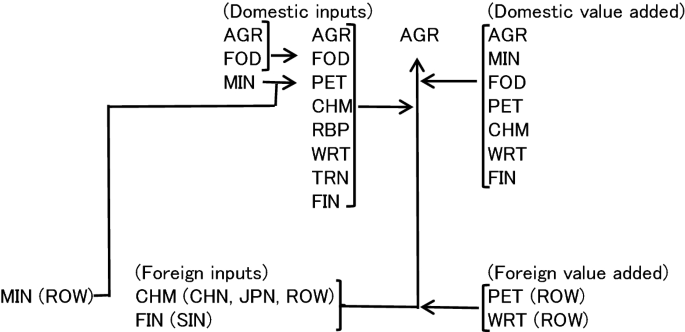
(source: calculated from the OECD’s ICIO tables, 2011)
In summary, these figures demonstrate the sequence of upstream transactions of goods and services induced by one unit of final demand for agricultural products. Additionally, the value-added activities that accompany the transactions of goods and services are recorded on the right-hand side of the figures, deriving the information from the corresponding sectors in the VA row in Tables 5, 6, and 7. For instance, the top left of Fig. 2 shows that the Thai agricultural sector received inputs from domestic sectors such as agriculture (9.1), food products (7.9), refined petroleum (4.1), chemicals (2.2), rubber products (0.6), financial intermediation (3.7), wholesale and retail trade (2.8), and transport (0.8) (the figures in parentheses are derived from Table 5). Among them, a value chain sequence, mining (from both Thailand and the ROW) → refined petroleum → agriculture, can be seen in the domestic input transactions. Simultaneously, value added is generated in the sectors that provide intermediate inputs (see the top right of Fig. 2).Footnote 12 Because a higher consumption of refined petroleum is considered to reflect a higher usage of agricultural machinery such as tractors and harvesters, the existence of such a sequence reflects a higher level of mechanization in the Thai agricultural sector.
Moreover, since chemical products, which include chemical fertilizers and pesticides, are critical inputs for agriculture, the sequence of chemicals → agriculture is also an important segment of the agricultural value chain, for which the major suppliers of chemicals were Thailand (2.2), Japan (0.6), China (0.5), and the ROW (0.5).
Figure 3 indicates the similarities in the structure of the value chains of Vietnam and Thailand, but a notable difference is that chemical inputs were relatively low in Vietnam (0.6). Furthermore, unlike Thailand, inputs from refined petroleum do not appear in Fig. 3.Footnote 13 Regarding foreign inputs, inputs from agriculture, food products, and wholesale and retail trade were relatively high, but neither chemicals nor refined petroleum was included in this category. These results suggest that there is still room to improve the productivity of Vietnam’s agricultural sector in terms of the use of chemicals and agricultural machinery, particularly those imported.
Fig. 3 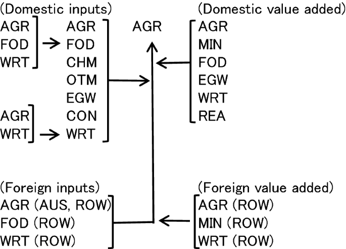
(source: calculated from the OECD’s ICIO tables, 2011)
Flow of upstream transactions: agricultural sector in Vietnam (2011). This figure is based on Table 6
The above structure is clearly shown in Fig. 4. As shown in Table 7, Cambodia had an extremely high value-added share in the agricultural sector (98.14). This result implies that Cambodia’s agricultural sector was highly self-sufficient and that its backward linkages with other sectors, including chemical inputs and refined petroleum, were extremely weak.Footnote 14, Footnote 15 As in other countries, a variety of industries were stimulated by agricultural output, but their volume was extremely small. However, it is still notable that the sequence of mining (Vietnam) → refined petroleum (Vietnam) → agriculture (Cambodia) was an important segment of Cambodia’s agricultural value chain, reflecting Cambodia’s strong linkages with the Vietnamese supply chain.
Fig. 4 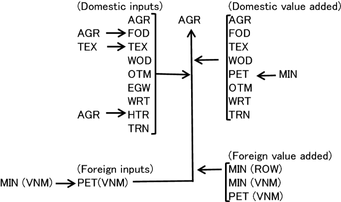
(source: calculated from the OECD’s ICIO tables, 2011)
Flow of upstream transactions: agricultural sector in Cambodia (2011). This figure is based on Table 7
-
2.
Downstream transactions
Figures 5, 6, and 7 are produced based on Tables 8, 9, and 10, respectively. In contrast to Fig. 2, Fig. 5 starts with one unit of value added (primary inputs) in agricultural products, which is subsequently used as an intermediate input for purchasing sectors such as food products. The outputs of the purchasing sectors are then used as inputs for other purchasing sectors such as hotels and restaurants, whose outputs are finally consumed by households. Consequently, these figures demonstrate the sequence of the downstream transactions of goods and services induced by one unit of value added (primary inputs) in the agricultural sector.
Fig. 5 Fig. 6 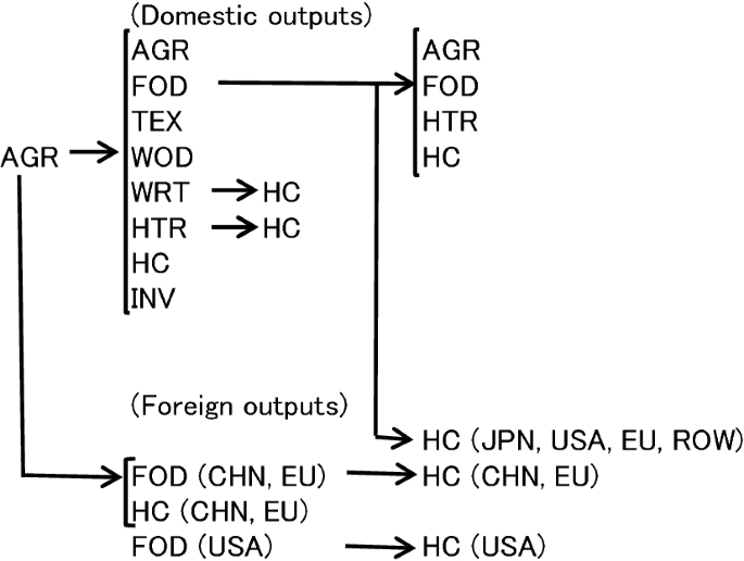
(source: calculated from the OECD’s ICIO tables, 2011)
Flow of downstream transactions: agricultural sector in Vietnam (2011). This figure is based on Table 9
Fig. 7 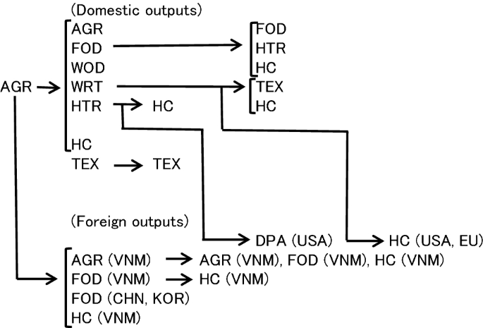
(source: calculated from the OECD’s ICIO tables, 2011)
Flow of downstream transactions: agricultural sector in Cambodia (2011). This figure is based on Table 10
Figure 5 shows that in Thailand, agricultural outputs were used as inputs for food products (35.6), agriculture (9.1), rubber products (7.7), wood products (1.7), textiles (1.5), hotels and restaurants (5.6), as well as final demand sectors such as household consumption (25.3) and changes in inventory (2.2). Among them, food products received the largest amount of agricultural input. Food products were then used as inputs for food products (6.2), agriculture (2.9), hotels and restaurants (3.6), and household consumption (13.9), as well as household consumption in Japan (1.5), the United States (1.2), the EU (1.2), and the ROW (1.8). Hotels and restaurants, whose services are finally consumed by households, were also important sales destinations for agricultural output.
Some agricultural outputs were exported to China (2.4) and Japan (1.0) as inputs for food products. Food products are consumed by households in these countries. Simultaneously, agricultural outputs were exported to China (1.0) as inputs for textiles.
Figure 6 shows that the basic structure of Vietnam’s agricultural value chain is similar to that of Thailand. As in Thailand, Vietnam’s food products were stimulated strongly by agricultural outputs (41.9), and sectors that were stimulated by food products inluded agriculture, food products, hotels and restaurants, and household consumption in both domestic and overseas markets. In Vietnam, however, the EU played a more significant role as a sales destination. Vietnam’s agricultural products were used by the food industry in the EU (2.2) and China (1.3), which then provided their outputs for household consumption in their home markets.
Figure 7 and Table 10 show that in Cambodia, overall transactions of goods and services induced by the agricultural sector were very small. First, this finding reflects the fact that the Cambodian agricultural sector, where a large percentage of agricultural output (71.0) was consumed by domestic households, had an extremely weak linkage with other sectors. Second, unlike Thailand and Vietnam, Cambodia’s food products did not stimulate household consumption abroad because the bulk of agricultural products were exported directly without further processing and were only used as inputs for agriculture (in Vietnam) and food products (in Vietnam, China, and Korea).
Third, some hotel and restaurant services, which received inputs from the agricultural sector (9.1), were directly purchased by residents from the United States (0.5). This finding reflects the fact that Cambodia attracted many foreign tourists who spent large amounts of money in local hotels and restaurants.
Finally, neighboring countries were becoming important trade partners of Cambodia. In particular, a substantial amount of Cambodia’s agricultural output was exported to Vietnam as an input for agriculture and food products, which then stimulated agriculture, food products, and household consumption in Vietnam. This also implies that lucrative markets, such as the EU, the United States, Japan, China, and Korea, have not yet been exploited by Cambodia’s agricultural industry.


4 Conclusions
This study introduced a method of value chain mapping that uses international input–output data. International input–output tables are one of the most comprehensive data sources that document all transactions of goods and services across national borders. The method of analysis introduced in this study combines the concept of value chain mapping with the input–output analysis technique, particularly the unit structure analysis and the supply-driven Ghosh model. The method clearly demonstrates that the value chain of a specific industry or commodity can be mapped with both the upstream and downstream transactions of goods and services traced along the chain. Furthermore, the method provides more comprehensive and detailed information on the sequences of value-adding activities along the chain than does the analysis of trade in value added.
The results of the analysis show that although the rapid progress of regional integration has affected the development of the agricultural value chain, there are still significant differences in terms of the internationalization of value chain activities. Thailand’s agricultural value chains are the most advanced and internationalized among the three countries in terms of upstream transactions. In particular, critical agricultural inputs such as chemicals and refined petroleum were procured from both international and domestic sources. However, Vietnam and Cambodia did not fully utilize opportunities to improve productivity by participating in GVCs. Specifically, Cambodia’s agricultural sector was highly self-sufficient, with little dependency on imported inputs.
In contrast, Thailand and Vietnam show diversified downstream transactions. In particular, food products produced using agricultural outputs were widely consumed by households in both domestic and international markets. In Cambodia, the overall transactions of goods and services stimulated by agricultural outputs were extremely small. Moreover, Cambodia’s agricultural output had no significant effect on household consumption abroad because of the underdevelopment of the food processing industry.
Although the method proved useful, there were some constraints regarding the data and methodology. First, it is desirable to construct more disaggregated data with a greater number of sector classifications, including for agriculture and related industrial sectors. Second, the current input–output data had an industrial activity-based sector classification, while a conventional value chain analysis concerns the business functions performed by firms, such as design, production, marketing, distribution, and support to the final consumer. Such a difference would be reconciled if input–output tables were constructed more in line with the concept of business functions.
Availability of data and materials
All data generated or analyzed during this study are included in this published article.
Notes
It holds that gross exports = value added exports (VT) + domestic content in intermediate exports that finally returns home (VS*) + foreign content in exports (VS) (Koopman et al. 2014). Thus, the ratio of value added exports to gross exports, called the VAX ratio (Johnson and Noguera 2012), is expected to decrease with the progress of vertical specialization.
In the following, if x, Z, f, and other symbols were replaced by the matrices or vectors that comprise only a single country, it would be equivalent to Ozaki’s unit structure analysis.
The value-added coefficient is the ratio of value added to total output.
For the repercussion mechanism of the Ghosh model, see Chapter 12 in Miller and Blair (2009). Miller and Blair also discuss the plausibility and mathematical relationship between the Leontief and Ghosh inverses.
The final demand coefficient is the ratio of final demand to total output.
In the ICIO tables, the final demand matrix for each country has 6 × \(m\) columns because the distribution of goods and services for final consumption is divided into \(m\) destination countries and six final demand columns (i.e., household consumption, non-profit institutions serving households, general government final consumption, gross fixed capital formation, changes in inventories, and direct purchases abroad by residents) for each destination country.
Although more recent ICIO tables (2005–2015: 2018 edition) were published by the OECD, this study will used the 2016 edition. This is because (i) the 2016 edition (1995–2011) is more suitable for exploring the impact of regional integration on the agricultural value chain since the early 1990s; and (ii) there are significant differences between the 2016 and 2018 editions in terms of, for example, the system of national accounts (SNA) and the international standard industrial classification (ISIC) used for the construction of the tables, so that they cannot be used interchangeably.
The VS measure indicates the degree of backward GVC participation at the country-sector level, while the VS1 measure provides the degree of forward GVC participation (Hummels et al. 2001; Koopman et al. 2014). This study, however, focuses on the VS measure, and the forward GVC participation will be discussed in connection with the downstream transactions of value chain mapping.
OECD (2013) shows that an industry with a high share of imported inputs displays, on average, higher productivity among OECD countries because foreign inputs embody more productive technology and local resources are allocated more efficiently. Specifically, increased productivity results from (1) a price effect—increased intermediate imports result in stronger competition and therefore lower prices for inputs; (2) a supply effect—increased imports enhance the variety of inputs available; and (3) a productivity effect—new intermediate inputs may spur innovation in the final goods sector by enhancing access to knowledge.
Exceptions to this are refined petroleum and wholesale and retail trade in the ROW. These sectors appear only in value added transactions because primary and service sectors tend to have higher value-added ratios than manufacturing sectors.
This implies that inputs from refined petroleum in Vietnam is below 0.4 units (i.e., the minimum value in Table 6).
A government official at the Ministry of Agriculture, Forestry, and Fisheries of Cambodia said to the author that the “chemicals used in agriculture are too little because of higher costs of imported agricultural chemical inputs and traditional farming systems, where the main purpose of farming is for household consumption.”.
Another possibility is that, as pointed out by Kuroiwa and Tsubota (2014), Cambodia’s external trade and linkages could be significantly underestimated because of its unofficial trade with neighboring countries, particularly Thailand and Vietnam.
In fact, there are potentially 509,796 (= (34 × 21)2) intermediate transactions plus 714 (= 34 × 21) value added transactions in Tables 5, 6, 7. On the other hand, the percentage shares of transactions recorded in the tables (= 100 × (intermediate plus value added or final demand transactions that appear in Tables 5, 6, 7, 8, 9, 10)/(all intermediate plus value added or final demand transactions induced by a unit of final agricultural outputs) are as follows: 64.7 percent (Table 5), 73.5 percent (Table 6), 95.8 percent (Table 7), 56.2 percent (Table 8), 68.4 percent (Table 9), and 82.0 percent (Table 10). Therefore, although the number of transactions covered in the tables is small, the percentage shares of transaction values are substantially high.
As an alternative criterion for selecting the transactions that appear in the tables, a threshold value (i.e. the minimum value) can be given to all the transactions. However, this alternative was not adopted, because there are significant differences in the transaction values between Cambodia and other countries.
References
Akamatsu K (1962) A Historical pattern of economic growth in developing countries. Dev Econ 1:3–25
Antràs P, Chor D (2013) Organizing the global value chain. Econometrica 81(6):2127–2204
Antràs P, Chor D, Fally T, Hillberry R (2012) Measuring the upstreamness of production and trade flows. Am Econ Rev 102(3):412–416
Borin A, Mancini M (2019) Measuring what matters in global value chains and value-added trade. In: World Bank policy research working paper, no. 8804
Daudin G, Rifflart C, Schweisguth D (2011) Who produces for whom in the world economy? Can J Econ 44(4):1403–1437
Fally T (2012) On the fragmentation of production in the US. University of Colorado. mimeo
Frederick S (2014) Combining the global value chain and global I-O approaches. In: A Paper Presented at the international conference on the measurement of international trade and economic globalisation, Aguascalientes, Mexico, 29 September–1 October 2014
Ghosh A (1958) Input-output approach to an allocation system. Econometrica 25:58–64
Hummels D, Ishii J, Yi K-M (2001) The nature and growth of vertical specialization in world trade. J Int Econ 54(1):75–96
Johnson RC, Noguera G (2012) Accounting for intermediates: production sharing and trade in value added. J Int Econ 86(2):224–236
Koopman R, Wang Z, Wei S-J (2014) Tracing value-added and double counting of gross exports. Am Econ Rev 104(2):459–494
Kuroiwa I, Tsubota K (2014) Economic integration, location of industries, and frontier regions: evidence from Cambodia. J Southeast Asian Econ 31(3):379–394
Miller RE, Blair PD (2009) Input-output analysis: foundation and extensions, 2nd edn. Cambridge University Press, New York
Miller RE, Temurshoev U (2017) Output Upstreamness and Input Downstreamness of Industries/Countries in World Production. International regional science review, 40(5):443-475.
OECD (2013) Interconnected economies: benefitting from the global value chains. Synthesis report. http://www.oecd.org/sti/ind/interconnected-economies-GVCs-synthesis.pdf (downloaded on 25 October 2015)
Ozaki I (1980) Structural analysis of economic development (3): determination of the basic structure of the economy [Keizai Hatten No Kouzou Bunseki (3): Keizai No Kihonteki Kouzou No Kettei]. Keio J Econ 73(5):720–748 (in Japanese)
Wang Z, Wei S-J, Yu X, Zhu K (2017a) Measures of participation in global value chains and global business cycles. NBER working paper 23222
Wang Z, Wei S-J, Yu X, Zhu K (2017b) Characterizing global value chains: production length and upstreamness. NBER working paper 23261
Acknowledgements
Not applicable.
Funding
This work was supported by JSPS KAKENHI [Grant Number 17K03749].
Author information
Authors and Affiliations
Contributions
The author read and approved the final manuscript.
Corresponding author
Ethics declarations
Ethics approval and consent to participate
Not applicable.
Consent for publication
Not applicable.
Competing interests
No competing interests of any sort.
Additional information
Publisher's Note
Springer Nature remains neutral with regard to jurisdictional claims in published maps and institutional affiliations.
Appendices
Appendix 1: Sector classification of the OECD ICIO table (Table 4)
Appendix 2: The VS share and its decomposition
The VS share represents the share of value added induced by exports but accrued to foreign countries. The methodology was originally developed by Hummels et al. (2001), and it was introduced into the analysis of trade in value added by Koopman et al. (2014).
Using Eq. (6), the VS share of sector j in country s (Eq. (40) in Koopman et al. 2014) can be expressed as
where \({\varvec{v}}_{\left( j \right)i}^{\left( s \right)r}\) represents the value added in sector i in country r induced by one unit of export demand for sector j in country s. Here, the VS share is expressed in percentage terms, so that it ranges from 0 to 100.
Furthermore, the \(VS_{\left( j \right)}^{\left( s \right)}\) share can be decomposed as follows:
-
1.
Share of foreign content by country of origin (country r):
$$VS_{(j)}^{(s)r} \;{\text{share = 100}} \times \sum\limits_{i = 1}^{n} {{\varvec{v}}_{(j)i}^{(s)r} } .$$(14) -
2.
Share of foreign content by sector of origin (sector i):
$$VS_{(j)i}^{(s)} \;{\text{share = 100}} \times \sum\limits_{r \ne s}^{m} {{\varvec{v}}_{(j)i}^{(s)r} } .$$(15)
Appendix 3: Input–output tables representing the unit structure
Tables 5, 6, 7 (Tables 8, 9, 10) are the input–output tables constructed based on Eqs. (5) and (6) (Eqs. (11) and (12)).
Each column in Tables 5, 6, 7 indicates how intermediate transactions and value-added (both domestic and foreign) are generated by each sector when one unit, which is actually normalized to 100 units in these tables, of final demand for agricultural outputs is given in Thailand (Vietnam, Cambodia). Transactions that occur outside Thailand (Vietnam, Cambodia) are recorded on the right-hand side of the tables. Since the transactions that occur within and outside the country are numerous, only the 25 largest transactions, whose values may differ depending on the country, are reported.Footnote 16 Footnote 17
In contrast, each column in Tables 8, 9, 10 indicates how the outputs are distributed to the respective sectors when one unit (which is normalized to 100 units) of value added (primary inputs) in agricultural products is given. The row sectors include not only intermediate sectors, but also final demand sectors; a large proportion of food products, for instance, are distributed to household consumption. As in the upstream transactions, downstream transactions that occur outside Thailand (Vietnam, Cambodia) are recorded on the right-hand side of the tables and only the 25 largest transactions are reported.
Rights and permissions
Open Access This article is licensed under a Creative Commons Attribution 4.0 International License, which permits use, sharing, adaptation, distribution and reproduction in any medium or format, as long as you give appropriate credit to the original author(s) and the source, provide a link to the Creative Commons licence, and indicate if changes were made. The images or other third party material in this article are included in the article's Creative Commons licence, unless indicated otherwise in a credit line to the material. If material is not included in the article's Creative Commons licence and your intended use is not permitted by statutory regulation or exceeds the permitted use, you will need to obtain permission directly from the copyright holder. To view a copy of this licence, visit http://creativecommons.org/licenses/by/4.0/.
About this article

Cite this article
Kuroiwa, I. Method of value chain mapping with international input–output data: application to the agricultural value chain in three Greater Mekong Subregion countries. Economic Structures 10, 6 (2021). https://doi.org/10.1186/s40008-021-00235-7
Received:
Revised:
Accepted:
Published:
DOI: https://doi.org/10.1186/s40008-021-00235-7