- Research
- Open access
- Published:
Health, inequality and income: a global study using simultaneous model
Journal of Economic Structures volume 7, Article number: 22 (2018)
Abstract
A simultaneous three-equation model is specified between GDP per capita (GDPc) level, infant mortality rate and health expenditures for 194 countries from 1990 to 2014. GMM-2SLS estimation results indicate that simultaneous decreasing infant mortality rate and increasing GDPc level effects are found in sample with three income level country groups. Health expenditures have larger than one elasticity when effects from GDPc level and number of doctors per capita are summed together. Increase in income inequality measured with GINI coefficient increases infant mortality rate in non-poor countries. We test for Kuznets’ hypothesis maintaining a positive GDPc level income inequality relationship in poor countries contrary to rich ones. Kuznets’ hypothesis is not rejected for poor countries with proposed ∩-shaped GDPc function on GINI that also identifies the negative income inequality effects on GDPc growth. In poorest countries, the possible Kuznets’ hypothesis and involved low-income high-inequality trap can be eliminated by raising health expenditures– GDPratio and with cost-effective health technology. Breaking the possible negative relationship between income inequality and health status in these countries makes health promotion policy and positive income–health path to develop smoothly.
1 Background
Today, the health of most people in the world depends on their ability to locally adopt health knowledge and health technologies that have been discovered and developed elsewhere. Life expectancy and infant mortality are major health status determinants that impact economic growth. OECD countries with higher life expectancies and low infant mortality rates have more economic development and higher standards of living than all other countries. However, unfortunately, only in recent times economists have realized that health is an important part of human capital formation sustaining economic growth and improvements in health status can be justified on purely economic grounds. Good health raises levels of human capital and this has a positive effect on individual productivity and human capital returns. Better health increases workforce productivity by reducing incapacity and the number of days lost to sick leave besides increasing the opportunities of obtaining better paid work. Although good health may be considered a form of human capital that has a beneficial effect on productivity, income also influences health in a positive way. The capacity to generate higher earnings facilitates an increase in the consumption of health-related goods such as adequate food, medicine and health care, which provide longer longevity. However, the income effects on health are not equally distributed. Wealthier people can provide higher investments in health capital although the marginal benefits are largest among the poorest. Thus, the simultaneous health–income relationship needs to be analyzed in a framework where income inequality also affects the health outcomes.
In response to this, we specify a simultaneous three-equation model between level GDP per capita (GDPc), health status (HS) and health expenditures per capita (HEc) for a data set of 194 countries in years 1990–2014. GDPc and HS determinations are also affected by income inequality, i.e., we propose that income inequality effects on GDPc (level and growth) and HS are depending on the income level of country. To obtain a compact approach on health and inequality effects on GDPc, the analysis is cast in the framework of Kuznets’ hypothesis maintaining a positive income inequality relationship for poor countries contrary to the rich ones. We argue that so-called low-income high-inequality trap can be escaped in the presence of Kuznets’ hypothesis by raising the health expenditures–GDP ratio and with cost-effective health technology. The argument is that the poorest countries can quite quickly do this, if improvements in their health status and inequalities create a push effect in the growth direction. This can happen easily when negative relationship between income inequality and health status is not present. However, often inequalities, low levels of health expenditures, high unemployment, low levels of education and labor productivity and detrimental health-related behavior in non-rich countries—all slow down or even hinder this important and urgently needed catch-up. Estimation results show that Kuznets’ hypothesis is still relevant for countries with low GDPc levels, i.e., low-income high-inequality trap is still present in the poorest countries blocking the catch-up. However, the modern version of hypothesis maintaining that income inequality has negative effect on the growth of GDPc is not rejected for countries with different levels of GDPc. Generally we show that a positive bidirectional health–income relationship is not rejected and that more equal income distribution decreases infant mortality rate.
The structure of paper is as follows. Sections 2 and 3 focus on the studies on health and inequality effects on economic growth. Section 4 analyzes the Kuznets’ hypothesis and gives the model to be estimated. In Sect. 5 the estimation results are given and discussed. Section 6 ends the paper with conclusion. Subsequently, appendices give the study variables with data resources, review of the relevant econometric methods and detailed estimation results.
2 Health and economic growth
In the second part of the twentieth century, child mortality rates and life expectancy improved throughout poor countries. Gwatkin (1980) and Deaton (2013) labeled this as the third of three great waves of mortality decline. Here the first, starting at the end of the nineteenth century, began in North and Western Europe and was then transmitted to North America. The second wave, beginning in the nineteen twenties, was in South and Eastern Europe. The rate of gain in life expectancy was even more rapid then than in the first wave. By the middle of the twentieth century, life expectancies in the South and Eastern Europe were close to those in the north and west. The third great wave was in the poor economies beginning after the Second World War and was aided by international public health efforts, particularly the Bretton Woods and UN institutions.
Gains in income were important for improving nutrition and funding along with better water and sanitation schemes. However, some countries made progress in reducing infant mortality even in the absence of such economic growth (Reinhart 1999). This health improvement came from the globalization of health and health care knowledge. More recently, the global infant mortality decline has depended on transmission of both conventional and advanced health care technology. Although they may be expensive, medical techniques diffuse more rapidly than changes in behavior, which respond slowly and unevenly to changes in knowledge about health risks (Aguayo-Rico et al. 2005). However, if one accepts the argument that health is largely determined by the transfer of technology and knowledge, the current state of mortality from any epidemic in any part of the world is evidence of the failure of globalization to transfer effective drug based technology and treatment from the rich countries to the poorer ones (Shastry and Weil 2002).
Partly as response to these new aspects of human capital a new family of theories of economic growth emerged in the 1980s that were better equipped to explain long-term growth (Romer 1986; Lucas 1988). Central to these models was the idea that technology was endogenous to the growth process. In the neoclassical growth models, the notion of growth as increased stocks of capital goods was codified in the Solow–Swan growth model. In contrast to these Lucas (1988) and Romer (1986) considered technology as endogenous and incorporated a new concept of human capital which had increasing rates of return. The focus shifted on increased human capital, learning and level of R&D activity. However, one saw still large variations in health between rich and poor countries contributed to differences in income and vice versa. Better health of workers meant higher productivity and less disparities of income which in their turn meant more spending causing improved health and longevity. So, there was a multiplier effect with better health. Similarly, the effects of exogenous health improvements like a vaccine that made workers healthier lead to a multiplier effect as healthier workers produced more output (Weil 2005, 2009). This “health view” assumed that income differences between the countries were mainly caused by different health environments. The “income view”, on the other hand, assumed that most differences between the countries had their roots in aspects of production that were unrelated to health, e.g., in physical capital accumulation or technology. Weil (2005, 2009) further showed that there was a link between poverty reduction and long-term economic growth that was impacted by health. From the early 1990s, the role of human capital (including health) was almost universally regarded as being indispensable for economic growth. Sustained growth depended on levels of human capital whose stocks increased because of better health and education, effective learning and training procedures. Without a labor force with some minimal levels of education and health, a country was incapable of maintaining a state of continuous growth (Rivera and Currais 2003).
The analysis and comparison of mortality patterns in several economies led Morand (2004) to suggest the theory of epidemiological transition. There were three basic patterns of transition in this theory, namely the classical or western model, the accelerated model, and the delayed one. These three patterns corresponded to three scenarios of i) endogenous transition during the neoclassical growth regime, ii) endogenous transition during the modern growth regime, and iii) transition triggered by exogenous factors. In an endogenous growth model output was produced by combining physical and human capital inputs, where agents could invest in health and education resulting in improvement of their human assets (Galor 2011; Van Zon and Muysken 2001). This, in turn, affected their lifetime utility positively. So, economic growth had a direct effect on health status and longevity which in turn impacted economic growth.
Empirical growth model estimates have generally showed the importance of health status on growth. A study by Lorentzen et al. (2008) regressed GDPc on the average child and adult mortality rates over the period 1960–2000. The study found a strong effect of mortality rates on income growth. Aghion et al. (2010) analyzed the relationship between health and growth across OECD countries using cross-country panel regressions. They found a significant and positive impact of health on growth and vice versa between 1940 and 1980. This study showed that between 1940 and 2000 average GDPc and average life expectancy among high-income countries achieved larger gains in GDPc but smaller increases in life expectancy than they did in low and middle-income countries. By combining both so-called Lucas and Nelson–Phelps approaches, they could show that achieving higher life expectancy had a positive significant effect on GDPc growth. It improved health standards and increased current productivity growth (“Lucas effect”), while higher health standards improved future productivity growth (“Nelson–Phelps effect”).
Bloom et al. (2004) showed that improvements in health increased output not only through labor productivity, but also through capital accumulation. There was a positive impact of health and health expenditures on income growth. There were four ways by which health impacted economic growth. It enhanced labor productivity, created a greater labor supply, acted as a catalyst for education and training that fostered higher skills, and called for more savings leading to more investment in physical and intellectual capital. Bloom and Canning (2008) further showed that health also affected prospective life spans and life cycle behaviors. To the extent that income was a consequence of health, investments in health were to become a priority. This argument for health as an investment good was particularly relevant since there were cheap and easily implementable health policies that could improve health dramatically.
According to Sachs (2001), rising health status drives economic growth. The lag between declines in mortality and fertility resulted in a baby boom generation that started a period of economic growth as they entered the workforce. Sachs (2001) called this “demographic dividend”. Health, (income) inequality and economic developments were endemically interrelated. Policies with regard to health spending influenced welfare of contemporary and next period’s generations which then influenced economic growth. The long-term demographic and economic data with regard to developed OECD countries showed that increase in general human capital during transition periods influenced the rhythm of economic growth permanently. As per capita income went up, the longevity of population increased. As longevity went up, savings and investment for education and retirement increased. This was supported by higher rates of private and public investments for health. This leads to capital accumulation, which in turn leads to the economies’ aggregate efficiency and levels of economic activities to go up (see also Casasnovas et al. 2005; Cervellati and Sunde 2009; Aisa and Pueyo 2006).
De la Croix and Licandro (1999) focused on an overlapping generation model with uncertain lifetime and endogenous growth. The model gave the positive effect of life expectancy on growth for economies with a relatively low life expectancy. However, this was negative in more advanced economies. The positive effect of a longer life on growth could be offset by an increase in the average age of the workers. Life expectancy affected growth directly, namely when the probability of dying young was high, the discount rate was also high making it optimal for people to start working early in their life and not to stay at school too long (Fogel 1994). When households had to decide the moment at which they would leave school to work, life expectancy became a central factor that affected the optimal length of education and hence the growth rate of the economy. So, the positive effect of a longer life on growth could be offset by an increase of the average age of the working population.
Bhargava et al. (2001) investigated the effects of health indicators such as adult survival rates (ASR) on GDP growth rates at 5-year intervals in several countries. The models for growth rates were estimated considering the interaction between ASR and lagged GDPc level. Endogeneity and reverse causality were considered. Average life expectancy in many developing countries was only 40 years in 1950 but increased to 63 years by 1990. Many factors like improved nutrition, better sanitation, innovations in medical technologies, and public health infrastructure increased life span. Further, life expectancy was strongly influenced by child mortality and low-cost interventions. Bhargava et al. showed that for the poorest countries, a 1% change in ASR was associated with an approximate 0.05% increase in economic growth rate. While the magnitude of this coefficient was small, a similar increase of 1% in investment/GDP ratio was associated with a 0.014% increase in growth rate. One could see ASR in poor countries reflected the levels of nutrition, smoking prevalence rates, infectious diseases, health infrastructure and factors like accidents leading to premature deaths. By contrast, differences in ASR in middle- and high-income countries were influenced by genetic factors and by access to and costs of preventive and curative health care. Because investments in skill acquisition in poor countries depended on the ASR, the years for which skilled labor remained productive were important for explaining economic productivity.
The empirical literature on the effect of health on economic development (Bloom et al. 2004; Webber 2002; Acemoglu 2011) focused on the labor productivity effects of health on economic growth where improvements in health lead to an increase in per capita income directly, as each individual was able to produce more per unit of labor input. On the other hand, the significance of the demographic variables in growth regressions was asserted by many other authors (Bloom et al. 2004; Sala-i-Martin et al. 2004). The fertility equation was found, e.g., by Schultz (1997). He considered the determinants of fertility to be education, income, employment, religion, nutrition, family planning and child mortality. Bloom et al. (2004) provided a summary of results of various studies that used life expectancy as a proxy for health in the analysis of the direct effect of health on education and economic growth (e.g., Barro and Lee 1984; Bhargava et al. 2001; Barro and Sala-i-Martin 2004; Sachs and Warner 1997; Blackburn and Cipriani 2002; Chakraborty 2004; Ehrlich and Lui 1991).
The role of health in economic development was analyzed via two channels in the paper by Finlay (2007), namely the direct labor productivity effect and the indirect incentive effect. The labor productivity hypothesis asserted that individuals who were healthier had higher returns to labor input. The incentive effect said that individuals who were healthier and had a greater life expectancy had the incentive to invest in education as the time horizon over which returns could be earned was extended. Education was the driver of economic growth, and thus, health played an indirect role in the model. Finlay’s results showed that the indirect effect of health was positive and significant.
Generally, the above results are, however, affected by income distribution—both directly and indirectly via its health effects. The relevant literature (see the reviews by Galor 2009; Aghion et al. 1999) shows that the inequality effects on economic growth could be substantial but diverse (Voitchovsky 2009). As different forms of inequality have a major impact on health status—on both infant mortality and life expectancy—the GDPc level and growth relationship between health status and must pay attention also to (income) in equalities.
3 Inequality and economic growth
Rising inequality is a concern of today. In advanced economies, the gap between the rich and poor is at its highest level in decades (Stiglitz 2013). Pervasive inequalities exist also with reference to access to education, health care and finance. Countries with higher levels of income inequality tend to have lower levels of mobility between generations, with parent’s earnings being a more important determinant of children’s earnings (Corak 2013). Redistribution has played an important role in cushioning market income inequality in mostly advanced economies. Many studies suggest that growing wealth inequality in advanced economies is largely driven by rising wealth concentration at the top (Piketty 2014; Saez 2014). An increase in income inequality can have both growth-promoting and growth-dampening effects. In their calculations, using data from 73 countries, Cornia and Court (2001) came to the conclusion that GINI coefficient value between 0.25 and 0.40 had a growth-promoting effect. At GINI coefficient value of 0.45 and above, an increase in income inequality had a growth-dampening effect.
A high level of income inequality impairs economy’s human capital insofar as low-income people do not have sufficient access to capital formation, health care and education. Typically, high level of income concentration leads to a situation where economic power is used to exert political influence to reduce taxes (Bernstein 2013). Decline in state revenues can cause reduction in investments in public health infrastructure and education. The resulting undersupply of public services dampens economic growth through a lack of public infrastructure and low productivity because of low expenditures (Galor 2011). On the demand side, a high degree of income inequality weakens the demand for goods and services. When increasing share of income goes to high-income households, the consequent savings and capital outflow causes less demand (Bernstein 2013). In less developed economies, savings can be available for investment, but sustaining consumer demand is missing. In highly developed economies, the level of capital stock is already high. If there is then a decline in consumer demand, there is no incentive for additional investment. Thus, growth in the economy’s overall capital stock weakens along with long-term growth potential. In the medium term, this trend leads to stagnation or even economic contraction. So, in sum, whether an increasing level of income inequality dampens future economic growth—weakening both the supply side (human and real capital) and the demand side—largely depends also on the economy’s GDPc level (Petersen and Schoof 2015).
Income and wealth distributions are systematically, albeit in nonlinear fashion, affected by the level of economic development. A lucid review of the “Kuznets school” is given by Piketty (1997), Deininger and Squire (1998), and Kanbur (2012). At a low level of GDPc, income and wealth distributions are wide but they change to become less wide when the economy reaches higher GDPc level (Kuznets 1955). The modern condensed version of this hypothesis says that if the income or wealth distribution is unequal, the rate of economic growth is low. However, this version abstracts from the fact that the relationship suggested by Kuznets is path dependent. Kuznets himself used pre-World War 2 time-series data for USA, UK and Germany and argued that the level of GDPc determined when the inequality–growth relationship was positive and when it was negative. Typically, at a low level of GDPc, one observed positive relationship between inequality and growth, while negative relationship prevailed at higher levels of GDPc. The latter results were expected when there were no obstacles for equal opportunity to human capital investment and productivity gains.
Generally, if capital had decreasing returns and capital markets were imperfect, the distribution of wealth mattered for GDPc level and growth. In such a situation, only redistribution and public intervention to capital markets supported higher economic growth because income and wealth redistribution created many new investment projects with higher marginal returns and effort supply (Aghion et al. 1999). Benabou (1996) and Lee and Roemer (1998) concluded that generally private (human capital) investment and inequality did not show monotone negative relationship. Benhabib (2003) showed that the hump-shaped relationship comparable to Kuznets’ hypothesis could be found for inequality–growth relationship. Typically, with more unequal distribution and high capital taxes growth was hampered.
There exists also the perspective of sociopolitical theories (Gupta 1990; Alesina and Perotti 1996; Benhabib and Rustichini 1996). One version maintains that a greater degree of inequality in wealth and income could raise the likelihood of poor people participating in highly destructive activities such as crime, rioting and revolution. The resulting instability and distrust in the entire economic system could then lead to a decline in investment incentives, which could hamper long-run economic growth. The studies by Perotti (1994, 1996), Alesina and Rodrik (1994), Persson and Tabellini (1994) and De Mello and Tiongson 2006 based on the median voter and mean income model, i.e., economic growth would be improved by a middle class that is sufficiently wealthy to vote for a low level of redistribution, found evidence of a negative relationship between inequality and economic growth. Moreover, the link between redistribution (e.g., the amount of taxes) and growth is found to be weakly negative or even positive. Forbes (2000) showed that a positive relationship between inequality and growth could be possible in the short- or medium-term when one was using high quality data for income inequality provided by Deininger and Squire (1996). She argued that it was more likely to be negative in the long-run while being significantly positive in the short-run (see also Li and Zou 1998; Halter et al. 2014).
Barro (2000) examined the relationship through three-stage least squares using the same inequality data as in Forbes (2000) with an extensive set of control variables to reflect the sociopolitical status of each country. Unlike Forbes (2000), however, his estimation results showed that the effect of inequality was insignificant once the equation included various explanatory variables representing the correlation between the degree of economic development and the inequality level. Barro showed that the effects of inequality on growth differed, depending upon stages of economic development across countries. The paper by Barro (2008) updated and extended his earlier work. International data confirmed the presence of the Kuznets’ curve that was relatively stable from the 1960s to the 2000s. A cross-country growth equation showed a negative effect of income inequality on economic growth, holding fixed a familiar set of other explanatory variables. This effect diminished as GDPc level rose and was even positive for the richest countries (see also Castello-Climent 2010). Neves et al. (2016) showed that the direction of growth effects also followed a certain time pattern: in the 1990s, most of the published studies found negative effects while at the beginning of this century, this tendency was reversed and empirical studies increasingly documented positive results. Cingano (2014) investigated the relationship between economic growth and inequality for data covering most of the OECD countries over the past 30 years. Different inequality measures in the growth equation were negative and statistically significant. He also evaluated the human capital accumulation theory and delivered evidence for human capital being a channel through which inequality could affect economic growth. For additional results on inequality effects on growth see, e.g., Herzer and Vollmer (2012), Kurita and Kurosaki (2011), Ostry et al. (2014), De Gregorio and Lee (2004), Lee and Son (2016), Baur et al. (2015) and Petersen and Schoof (2015).
Available evidence on the links between inequality and social mobility is also largely based on cross-country correlations showing a negative relationship between inequality and inter-generational earnings mobility in a subset of OECD countries (D’Addio 2007; Corak 2013). Recent work by Chetty et al. (2014) based on millions of administrative data on income mobility in the USA finds that (upward) mobility is robustly negatively correlated with income inequality (and positively with school quality).
A common drawback of most empirical studies analyzing the growth–inequality relationship lies in a possible misspecification of the model. They do not account for the hypothesis that the effect of inequality on economic growth could be nonlinear depending on the stage of development (i.e., the level of GDPc) and the initial level of inequality. The analysis by Kolev and Niehues (2016) delivers evidence in favor of this hypothesis. Economic growth is negatively correlated with net income inequality for countries with low initial level of GDPc. However, the effect becomes weaker with increased GDPc level and even positive for the case of developed countries. In addition to Kuznets’ hypotheses, the human capital accumulation theory can motivate nonlinear inequality effects on economic growth.
Banerjee and Duflo (2003) stress the fact that the relationship between change in income inequality and GDPc growth is highly nonlinear and find empirical support for their conjuncture by using partial linear models. This has naturally implications for Kuznets type analysis although Banerjee and Duflo (2003) anchor their analysis mostly to a political economy model. Their results on partially linear models imply that there exists nonlinearity, and for mostly data points negative relationship, between growth and changes in GINI coefficients for 45 non-poor countries in years 1965–1995 with non-overlapping five-year period panels. They use controls taken from Barro (2000) and Perotti (1996). They sum up that changes in the inequality variable are associated with lower growth in the short run, independent of the direction of these changes. Accordingly, they argue that this nonlinearity can explain why the results of empirical research have been so different under the constraint of linear specification. Chen (2003) even finds a statistically significant quadratic term in the regression analysis pointing toward an inverted U-shaped relationship between inequality and economic growth.
The study by Voitchovsky (2005) has the central hypothesis that top-end inequality encourages growth while bottom-end inequality retards growth. This is explored using a standard growth model and a set of explanatory variables to control for inequality at the top and the bottom ends of the income distribution simultaneously. A panel GMM estimation is undertaken on a sample of industrialized countries, using data from the Luxembourg Income Study (2003) which indicates that inequality at different parts of the distribution does have different implications for growth, i.e., the profile of inequality is also an important determinant of economic growth. Top-end inequality appears to have a positive effect on growth, while inequality further downs the income distribution appears to be inversely related to subsequent growth. These findings highlight possible limitations of an exploration of the impact of income distribution on growth using a single inequality statistic.
Dominica et al. (2008) and Neves et al. (2016) conduct a meta-analytic reassessment of the effects of inequality on growth. The former points out that the magnitude of the estimated effect of inequality on growth in the literature depends crucially on the estimation method, data quality and sample coverage. Studies using panel fixed effects estimators seem to report stronger effect of inequality on economic growth than cross-sectional results. Overall, the results of the meta-analysis by Dominica et al. (2008) show that the inequality effect on growth tends to be negative and more pronounced in less developed countries. Neves et al. (2016) extend the meta-analytic reassessment to more recent studies and show that the empirical literature on the inequality–growth nexus is biased toward statistically significant results. As the authors stress, this makes the empirical effect of inequality on economic growth seem larger in absolute terms than what it is actually.
From policy perspective, the current level of results is too mixed. There is no one-size-fits-all approach to tackling inequality effects on GDPc. One neglected issue is that growth rate of GDPc and income inequality affects each other simultaneously (Baumol 2007; Lundborg and Squire 2003; Huang et al. 2009). It is not only the level of GDPc that conditions the income inequality but the growth rate also matters. In the following these questions are cast back in the framework of Kuznets’ hypothesis to have a systematic approach to build simultaneous model between GDPc, health level and health expenditure where inequality plays an important role.
4 Models, data and methods
4.1 Kuznets approach
In following we propose a simultaneous three-equation model for GDP per capita level (or GDPc growth), health status (HS) measured with infant mortality rate (IM) and health expenditures per capita (HEc) for data set of 194 countries in years 1990–2014. Income level and inequality (INEQ) determine IM that subsequently affects the level of HEc with income level. GDPc is also determined by typical labor or population, educational and technological input variables. In order to analyze GDPc growth effects we propose a similar simultaneous model GDP per capita growth rate (ΔlnGDPc). Models are given in details in Sect. 4.3.
Nonlinear Kuznets’ GDPc effects with income inequality depending on the level of GDPc must be specified into the model. This happens by estimating the model for three different GDPc level country groups. The nonlinear income level effects on inequality allow us to analyze the Kuznets’ hypothesis in details that is often neglected in the literature. Because our system model includes also linked equations for health status and health expenditures we argue that low-income high-inequality trap implied by Kuznets’ hypothesis can be escaped under suitable conditions by rising the health expenditures–GDP ratio and with cost-effective health technology. This happens even if the negative inequality–health status relationship is still valid in the poorer countries. In practice we test for Kuznets’ hypothesis maintaining a positive income inequality relationship for poor countries contrary to rich countries in the model where we estimate also the empirical linkages between GDPc, HS and HEc variables.
4.2 Health-poverty trap and Kuznets hypothesis in income–health model
Main argument behind our empirical model is the following stylized figure (see also Shin 2012). It shows that
-
(1)
if a country is in the low-GDPc high-inequality trap (R1), it can escape from it by increasing inequality (INEQ) that sustains higher GDPc, and
-
(2)
after some high level of inequality GDPc increases only if inequality starts to decrease, but
-
(3)
if the country increases its relative investment in health (i.e., HE/GDP –ratio increases: A \(\to\) A*), and the new level of health expenditures (HE) is utilized efficiently to raise country’s health status (HS), then the country will escape from the low-GDPc high-inequality trap (R2) (see Fig. 1).
Fig. 1 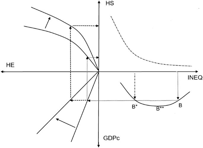
Determination of health status (HS) with Kuznets’ curve and health expenditures (HE) with given income inequality levels (INEQ)

Note that negative and monotone health status and inequality relationship (HS–INEQ) with large given inequality is the main part of our argument. It can be supported with many arguments, but empirically it is still valid for the majority of poor and low-income countries (see, e.g., Linden and Ray 2017; Deaton 2003, 2013). Thus, we exclude from the analysis the case of poor country with equal income distribution. Note also that Kuznets’ hypothesis is not necessary for our policy alternative (increases in HE/GDP and HS/HE ratios) to work out successfully. Hypothesis makes it only harder way to happen as the way out of trap is not a direct one. The results with Kuznets’ hypothesis speak for big jump—health policy alternative with large exogenous productive investments in health services and technology with some short-run GDPc reductions to find the low inequality but later on a higher GDPc position. If GDPc-INEQ curve is monotonic and negative (less INEQ and more GDPc), the small-step policy will work out smoothly without rising inequality. If we have monotonic positive GDPc-INEQ curve (more INEQ and more GDPc) it leads in progress to cyclical GDPc long-run solution (see “Appendix 1”) that the active health promoting does not make less volatile.
Note that the above model with related policy options and arguments was based on the modern reading of Kuznets’ hypothesis, i.e., possible causation goes from inequality to level and to growth of GDP per capita. The original hypothesis was more the opposite one noticing that first the level of GDPc determines the income and wealth inequalities that must increase to give the way to the growth, and later on the growth is hampered if the inequalities are too large. In more formal way this means that inequality is ∩-shaped function of GDPc like
with b > 0 and d < 0. To express this as inverse function of INEQ is a difficult task and we don’t pursuit in that direction here. Instead, we analyze what can be obtained from the function
We have added time to variables to get the growth presentation of equation, i.e.,
The negative inequality–growth relation favored by modern literature is determined by conditions: \(\beta > 0{\text{ and }}\delta < 0\) for given (positive) value of dINEQ/dt and large values of INEQ. However, note the complex nonlinear relationship between the time change of GDPc, time change in INEQ, and the level of INEQ. Thus, with time-series observations the linear growth regressions on the level of INEQ are biased if the true relationship is nonlinear (Banerjee and Duflo 2003)
The first derivate of GDPc with respect to INEQ (or \(\frac{{{\text{d}}GDPc/{\text{d}}t}}{{{\text{d}}INEQ/{\text{d}}t}}\) presentation of the above result) gives result:
i.e., when \(\beta > 0{\text{ and }}\delta < 0\) change in GDPc (with respect to positive change in INEQ) is positive when INEQ is not above IE** (Fig. 2, right panel). When we compare this outcome to “classical” Kuznets’ proposition, we observe similarities between the models as long as IE < IE* with low values of GDPc (see Fig. 2, left panel).

Kuznets curve and ∩-shaped GDPc function of inequality
Both models imply that inequality must rise to sustain the GDPc level first (the classical Kuznets hypothesis), but for Kuznets’ curve a radical change happens at some level of GDPc (and INEQ) that turns GDPc–INEQ relationship negative. In our model this is also found at high values of INEQ but level of GDPc decreases after it, i.e., any low INEQ–high GDPc solutions are not found in our model. The difference between the models comes more evident when we look at models in derivate terms dGDPc/dINEQ. In Kuznets’ model the derivate is infinite at the turning point value IE* (sometimes called also as a catastrophe point) implying that derivate is \(\to + \infty {\text{ and}} \to - \infty\) very close to it. Empirically this is not a reasonable outcome. However, in our model there exists a well-determined region not identified by original Kuznets’ curve below IE** level where inequality rises but positive (time) change of GDPc decreases to zero giving negative relation between positive growth rate of GDPc and INEQ. However, the GDPc level and INEQ relationship is still positive up to point IE**. In practice this means that some implications of Kuznets’ hypothesis and curve can be estimated with our ∩-shaped function
Case of \(\beta > 0{\text{ and }}\delta < 0\) is here relevant—before the maximum point of our ∩-shaped function is obtained—for the modern GDPc growth literature. Note that some features of the upper arm of Kuznets’ curve is obtained also with \(\beta > 0{\text{ and }}\delta < 0\) values when INEQ is large, i.e., negative relationship between INEQ and GDPc level. To sum up we argue that our GDPc–INEQ model gives an efficient way to test Kuznets–hypothesis for countries at different GDPc levels. Next this is done with simultaneous model in the context of health status and expenditure relationships with GDPc.
4.3 Health–income simultaneous equations model
As inequality is only one of the factors of economic growth, we can see empirically quite different inequality–growth correlations with, e.g., income GINI coefficients and GDPc growth rates when the other growth factors are neglected. Thus, without paying attention to the starting level of GDPc, human capital, and other growth inputs these correlations are misleading. We focus next on simultaneous health expenditure and status relationships with level and growth of GDPc where income distribution determines both health status and GDPc.
The following three-equation model captures the interlinked health and growth effects that are conditioned with prevailing income inequality in economy. The first equation is a typical empirical GDPc level equation based on production function that is augmented with economy’s health status (HS) and second-order polynomial in income inequality to measure its nonlinear GDPc effects. Population and educational variables (POP and EDUC) measure the effects of labor and human capital inputs on income. Variable TECH stands for the capital input measured as the change in nation’s technological advance. The second equation gives the determination of nation’s health status related to per capita GDP level, inequality and other health improving (exogenous) variables X1. Finally, health expenditures per capita (HEc) are determined by GDPc level, health status and some health expenditure-related (exogenous) variables X2. Thus, in general terms we argue that the income level (and growth) of economy is determined simultaneously with its health status and health expenditures. This means that in the model at least variables \({ \ln }GDPc, \, \Delta { \ln }GDPc\),\({ \ln }HS,\) \({\text{and}}\;{ \ln }HEc\) are endogenously determined. The structure of the model is identifiable and needs instrumental variable (IV) estimation approach.
Figure 2 and the above model are based on Kuznets’ hypothesis arguing that the relation between the GDPc level and inequality is hump-shaped. However, the more recent modeling (see Sect. 3) has focused on the growth rate and inequality. Albeit this growth formulation was easily derived in the preceding section in Kuznets framework, the modern theory and empirical literature have neglected the Kuznets’ approach too often. Thus, we follow partly here the Kuznets’ formulation prosed by Shin (2012) that the level of GDPc conditions also the inequality effects on GDPc growth rate, i.e., in poor countries inequality growth effects can be positive but in more advances countries they are negative. To get also more direct results comparable with modern literature, the first equation in our simultaneous model has now the following form
where we expect have positive sign for d2 poor countries, and negative sign is found in rich countries. To test this and the general nonlinear Kuznets’ approach, we divide our data (194 countries) in three income groups in 1995–2014 period:
-
S1: countries that average GDPc level was less than 1000US$,
-
S2: group countries with GDPc level in margins 1000–10,000US$, and
-
S3: group countries with GDPc level in the above 10,000US$.
4.4 Estimation strategy
To avoid the evident endogeneity of almost all variables in growth process modeling, we used the following approach. First, all our modeling variables are measured with the mean values of country specific variable values in period 1995–2014 (20 years: \(\bar{\varvec{Y}}_{i} ,\bar{\varvec{X}}_{i} )\). This makes the measurements independent of cyclical effects, and we can focus on average the long-run results. Second, we use means of variable measurements from period 1990–1994 as additional and instrument variables in model estimation. Thus, our instrumentation leans to pre-determination of variable values in relation to model estimation period. Variables dated at the beginning of sample period 1990–1994 reduce the problem of endogeneity. Note that if the variables are highly persistent endogeneity may still persist. Thus, we argue that (a) variable set \((\bar{\varvec{Y}}_{i, - 1} ,\bar{\varvec{X}}_{i, - 1} )\) from period 1990–1994 does not correlate with model errors \((\varvec{\varepsilon}_{1i} ,\varvec{\varepsilon}_{2i} ,\varvec{\varepsilon}_{3i} )\) in period 1995–2014, and (b) our additional instrument variables \((\bar{\varvec{Z}}_{i} ,\bar{\varvec{Z}}_{i, - 1} )\) do not correlate with model errors and not with left-hand-side endogenous variables, i.e., we have \(E[(\varvec{\varepsilon}_{1i} ,\varvec{\varepsilon}_{2i} ,\varvec{\varepsilon}_{3i} )|\bar{\varvec{Z}}_{i} ,\bar{\varvec{Z}}_{i, - 1} ] = 0\) and \(E[\bar{\varvec{Y}}_{i} |\bar{\varvec{Z}}_{i} ,\bar{\varvec{Z}}_{i, - 1} ] = 0\).
These conditions put high pressure for finding proper instrument variables that are not ill-conditioned by weak instruments and endogeneity. “Appendix 2” gives a more detailed description of methods used. However, we note that our \((\bar{\varvec{Z}}_{i} ,\bar{\varvec{Z}}_{i, - 1} )\) set compromises of values of alcohol consumption per capita (AC), percentage of population using improved drinking water source (AW), geographic area of country in km2’s (AREA) and means of GDPc level and growth of countries having the same level of development as country i (GDPc_iv). The last one is advocated by Pritchett and Summers (1993) as a valid instrument in this context. Thus, we argue that our endogenous left-hand-side variables \({ \ln }GDPc, \, \Delta { \ln }GDPc,{ \ln }HS\) measured with infant mortality (lnIM), and lnHEc measured with total health expenditures per capita are not necessarily affected by values of variables AC, AW, AREA and GDPc_iv in period 1995–2014 \((\bar{\varvec{Z}}_{i} )\) and by their period 1990–1994 values \((\bar{\varvec{Z}}_{i, - 1} )\). For example, in the above GDPc level equation the values of chosen instruments are independent of variable GDPc values but they affect the HS (infant mortality rate) values. Thus, e.g., using pre-determined period 1990–1994 mean values of the percentage of population using improved drinking water source (AW−1 or lnAW−1) as an instrument for IM is a natural choice in this equation but we also argue that it will not directly affect the value of GDPc.
5 Results
Table 1 reports the GDPc level GMM-2SLS estimation results for the model variables with main interest of this study. More detailed information on data used and estimation results is found in “Appendices 3 and 4”.
5.1 Health status (IM) effects on GDPc and HEc
Health status measured with infant mortality (lnIM) has a negative effect on the level GDPc. Largest effects are found in the poor countries with less than 1000US$ per capita income with coefficient value of − 1.32. Interestingly we found statistically negative effects also in rich countries (− 0.361). In the middle-income countries 10% increase in infant mortality rate decreases the level of GDPc with 7.56%. Contrary to these significant results, in both statistical and economic terms, we found only health status (IM) effects on health expenditures (HEc) in rich countries. A 10% increase in infant mortality rate increases health expenditures by 1.64%.
5.2 Income level (GDPc) effects on HS and HEc
In lnIM equation the level of GDPc decreases most effectively infant mortality in rich countries. A 10% increase of GDPc reduces the infant mortality rate by 6.4%. In poor countries the effect is only 1.78%. In InHEc equation income effects on health expenditures are largest in the middle-income countries (0.967). However, if we pay attention to the number of doctors per population (lnDOC) as part of health expenditures, the sum of these health expenditure elasticities is smallest in poor countries. Note, however, that in all country groups the sum of elasticities of GDPc and DOC on HEc is numerically above one.
From the policy perspective these results mean that (marginally) healthier people (i.e., reduced IM in lnGDPc equation) generates more income in poor countries compared to rich countries but when the level of GDPc is large enough, the wealth effects (GDPc in lnIM equation) increase health more effectively in richer countries than in poor countries. Health policy to reduce infant mortality seems to rise health expenditures (HEc) only in rich countries. However, GDPc level together with number of doctors per capita generate health expenditures in same magnitudes with respect to given level of GDPc in all income levels. These results may be an indication of poor efficiency and different targets for health expenditures in non-rich countries. In sum, if only one policy option is allowed then policy to reduce infant mortality is still a cost-effective policy alternative. For example, in the poor economies the net effect between GDPc and IM in lnGDPc and lnIM equations is large. A 10% reduction in IM means (ceteris paribus) a 13.2% increase in GDPc that sustains a lower IM rate with an estimated value of 2.34% \((13.2 \times 0.178)\). However, the (income) inequality effects on GDPc and IM may make this less evident.
5.3 Income inequality (GINI) effects on GDPc and HS
The GINI coefficients result in lnGDPc equation shows that nonlinear inequality effects (Kuznets’ hypothesis) on GDPc are found only in poor countries. We obtain ∩-shaped GINI outcome on GDPc level. As the GINI coefficients have values in range of 40-70 in poor countries, this means that our estimate for GDPc–INEQ relationship is hump-shaped (see Fig. 3). Estimation results for infant mortality rate (lnIM equation) show that in middle- and high-income countries increase in income inequality affects health status adversely, i.e., higher IM rate. Surprisingly in the poor economies (S1 group countries) this is not found. In these countries there is an indirect inequality effect on infant mortality rate: increase in GDPc level happens most likely with increasing inequality but only the GDPc increase lowers infant mortality rate that is not directly affected by GINI. Thus, the problem of infant mortality in poor economies is not so much caused by the income inequality but by the low level of GDPc.

Determination of health status (HS) in poor countries with Kuznets’ curve identified with ∩-shaped function and health expenditures (HE)
From the policy perspective this result is interesting. Now for a poor country with large inequality increases in HE/GDPc and HS/HE ratios lead to higher level health status. However, this can also happen with less inequality (compare points B and B* in Fig. 3). Between them we find an optimum value of inequality B** that provides the highest level of GDPc. Note that if HS–INEQ relation with typical shape as depicted in Fig. 3 would be valid here this would mean that quite moderate policy increase in HE/GDP or HS/HE ratio would move us from B to B* or to B**. However, the ∩-shaped GDPc–INEQ relationship allows not for a permanent trajectory with less income inequality and higher GDPc level. Only way to escape this trap is to hold to the health policy that raises health status and sustains eventually for higher GDPc level that breaks the ∩-shaped GDPc–INEQ relationship and allows for less inequality.
5.4 IM and income inequality (GINI) effects on GDPc growth
\(\Delta lnGDPc\) equation estimation results with linear effects of the GINI coefficients are given in Table 2. First, we observe that infant mortality rate has a positive but statistically insignificant effect on economic growth in all income groups. However, we find for all income level groups that larger income inequality (GINI) predicts less GDPc growth rate. The growth-reducing effect is largest in rich countries. For the poor countries significant negative estimate value of − 0.0009 means that these countries can be located on upper Kuznets’ curve arm and also left from the point IE** in Fig. 2.
When comparing the above GMM-2SLS results with SURE and GMM system results (obtained upon request), we observe that there exist larger differences between GMM-2SLS and SURE results than between GMM-2SLS and GMM system results in terms of point estimates and their SEs. As expected GMM system estimates are more efficient than GMM-2SLS estimates. However, the estimate and efficiency differences are not large enough in most cases to make above inferences with GMM-2SLS redundant. Also according to tests found in “Appendix 4” it is shown that our choice of instruments is valid one.
5.5 Endogenous income inequality effects
Basically, the Kuznets' hypothesis says that income level determines income distribution. The endogeneity of GINI coefficient is evident in this case. Next we do not propose an additional equation in the model for GINI variable but we estimated the above models treating GINI also as endogenous variable. Results in Tables 6, 7 and 8 (in “Appendix 4”) show that significant results with endogenous GINI were hard to obtain. Some results are still noteworthy. GMM C test rejects for poor countries the null alternative of exogenous GINI (see Table 6 in “Appendix 4”) for dlnGDPc equation, and the sign of GINI variable coefficient estimate is positive with 5% level. A clear increasing inequality effect on infant mortality is now also found for the poor countries in lnIM equation. However, in lnGDPc equation the estimates for second-order polynomial of GINI are very imprecise for all country groups. We take this as evidence of difficulty of finding proper instruments for endogenous GINI variable. The first-stage equation results in lnGDPc equation for GINI and GINI2 show the evidence of weak instruments. We leave the further analysis with endogenous GINI variable for future research.
6 Conclusions
Income–health relationship is in the core of health economic analysis—at both micro- and macro-levels. We analyzed the simultaneous relationships between health status measured with infant mortality rate and GDPc level and GDPc growth in the presence of income inequality variable (GINI) in infant mortality and income equations. System model included also equation for determination of health expenditures (HEc). Our sample consisted of data set of 194 countries in years 1990–2014. Cross section of country mean values of relevant variables in period 1995–2014 was used as estimation sample. Year 1990–1994 mean values were used as instrument variables with addition to some other variables. The cross-sectional data were divided into three country groups based on the mean GDPc level values during the sample period 1995–2014. This was done in order to test for Kuznets’ hypothesis maintaining a positive nonlinear relationship between GDPc level and income inequality in poor countries contrary to the rich countries.
Our GMM-2SLS estimation results indicated that the simultaneous positive infant mortality rate and GDPc level effects are found in all country groups sustaining decrease in mortality rate with an increase in GDPc level with positive feedback effect from lower mortality rate to GDPc. Increasing income inequality measured increased infant mortality rate. However, positive GDPc growth effects from infant mortality rates were not found. Health expenditures had larger than one elasticity when effects from GDPc level and number of doctors per capita were summed together.
We argued that for poor countries the low-income high-inequality trap can be also escaped in the presence of Kuznets’ hypothesis by rising the health expenditures–GDP ratio and with cost-effective health technology. This happens easily if the negative health status–inequality relationship is not valid or if the countries’ have positive nonlinear GDPc level dependence on income inequality with decreasing curvature. This was identified with ∩-shaped GDPc function on GINI coefficient. Both of these conditions were found in our sample only for the poorest countries and not rejecting the Kuznets’ hypothesis. However, the negative income inequality effects on growth of GDPc were found in all income level country groups. Weak tentative IV results with endogenous GINI did not support the Kuznets’ hypothesis for any country income level group and only significant, albeit positive, GINI effect on growth of GDPc was found for the poor countries.
From the economic growth policy perspective, our results mean that the policy to combine exogenously determined fight against infant mortality and income inequality means higher GDPc level in long run. In the poorest countries Kuznets’ hypothesis and low-income high-inequality trap may still be present but these can be avoided by breaking the possible negative relationship between income inequality and raising health status with the suggested policy. If this is not possible the positive income–health relationship will eventually make income inequality as obstacle to growth as the higher GDPc levels are reached.
References
Acemoglu D (2011) Thoughts on inequality and the financial crisis. Presentation at the American Economic Association Annual Meeting, 7 Jan 2011
Aghion P, Caroli E, García-Peñalosa C (1999) Inequality and economic growth: the perspective of the new growth theories. J Econ Lit 37(4):1615–1660
Aghion P, Howitt P, Murtin F (2010) The relationship between health and growth: when Lucas meets Nelson–Phelps. NBER Working paper series: 15813
Aguayo-Rico A, Guerra-Turrubiates IA, de Oca-Hernández RM (2005) Empirical evidence of the impact of health on economic growth. Issues Political Econ 14:1–17
Aisa R, Pueyo F (2006) Government health spending and growth in a model of endogenous Longevity. Econ Lett 90:249–253
Alesina A, Perotti R (1996) Income distribution, political instability and investment. Eur Econ Rev 40(6):1203–1228
Alesina A, Rodrik D (1994) Distributive politics and economic growth. Q J Econ 109(2):465–490
Banerjee AV, Duflo E (2003) Inequality and growth: What can the data say? J Econ Growth 8(3):267–299
Barro RJ (2000) Inequality and growth in a panel of countries. J Econ Growth 5(1):5–32
Barro RJ (2008). Inequality and growth revisited. Working paper series on regional economic integration no. 11, Asian Development Bank, pp 1–24
Barro RJ, Lee J-W (1984) Sources of economic growth. Carnegie-Rochester Conf Ser Public Policy 40:1–46
Barro RJ, Sala-i-Martin XI (2004) Economic growth. The MIT Press, Cambridge
Baumol WJ (2007) On income distribution and growth. J Policy Model 29:545–548
Baur M, Colombier C, Daguet S (2015) Ungleiche Einkommensverteilung hemmt Wirtschaftswachstum. Die Volkswirtschaft-Das Magazine der Wirtschaftspolitik 1–2(2015):8–11
Benabou R (1996) Inequality and growth. NBER Macroecon Annu 11:11–74
Benhabib J (2003) The tradeoff between inequality and growth. Ann Econ and Finance 4:329–345
Benhabib J, Rustichini A (1996) Social conflict and growth. J Econ Growth 1(1):125–142
Bernstein J (2013) The impact of inequality on growth. Washington, DC
Bhargava A, Jamison DT, Lau LJ, Murray CJL (2001) Modeling the effects of health on economic growth. J Health Econ 20:423–440
Blackburn K, Cipriani GP (2002) A model of longevity, fertility and growth. Journal of EconomicDynamics and Control 26(2):187–204
Bloom DE, Canning D (2008) Population health and economic growth. Commission on Growth and Development working paper no. 24. The International Bank for reconstruction and development/The World Bank on behalf of the Commission on Growth and Development, Washington D.C., pp 1–25
Bloom DE, Canning D, Sevilla J (2004) The effect of health on economic growth: a production function approach. World Dev 32(1):1–13
Casasnovas GL, Rivera B, Currais L (eds) (2005) Health and economic growth findings and policy implications. The MIT Press, Cambridge, pp 1–385
Castello-Climent A (2010) Inequality and growth in advanced economies: an empirical investigation. J Econ Inequal 8:293–321
Cervellati M, Sunde U (2009) Life expectancy and economic growth: the role of the demographic transition. Discussion Paper No. 4160, Institute for the Study of Labor, pp 1–51
Chakraborty S (2004) Endogenous lifetime and economic growth. J Econ Theory 116(119):137
Chen BL (2003) An inverted-U relationship between inequality and long-run growth. Econ Lett 79(2):205–212
Chetty R, Hendren N, Kline P, Saez E, Turner N (2014) Big data in macroeconomics: new insights from large administrative datasets Is the United States still a land of opportunity? Recent trends in intergenerational mobility. Am Econ Rev Pap Proc 104(5):141–147
Cingano F (2014) Trends in income inequality and its impact on economic growth. OECD SEM working paper 163
Corak M (2013) Income inequality, equality of opportunity, and intergenerational mobility. J Econ Perspect 27(3):79–102
Cornia GA, Court J (2001) Inequality, growth and poverty in the era of liberalization and globalization. Policy Brief 4 of the UNU World Institute for Development Economics Research (UNU/WIDER), Helsinki 2001
D’Addio AC (2007) Intergenerational transmission of disadvantage: mobility or immobility across generations? OECD social, employment and migration working papers 52, pp 1–112
De Gregorio J, Lee JW (2004) Growth and adjustment in East Asia and Latin America. Economia 5(1):69–134
De la Croix D, Licandro O (1999) Life expectancy and endogenous growth. Econ Lett 65:255–263
De Mello L, Tiongson E (2006) Income inequality and redistributive government spending. Public Finance Rev 34(3):282–305
Deaton A (2003) Health, inequality, and economic development. J Econ Lit 41(1):113–115
Deaton A (2013) The great escape; health, wealth, and the origins of inequality. Princeton University Press, Princeton
Deininger K, Squire L (1996) A new data set measuring income inequality. World Bank Econ Rev 10(3):565–591
Deininger K, Squire L (1998) New ways of looking at old issues: inequality and growth. J Dev Econ 57:259–287
Dominica LD, Floras RJGM, Groot HLF (2008) A meta-analysis on the relationship between inequality and economic growth. Scottish J Political Econ 55:654–682
Ehrlich I, Lui F (1991) Intergenerational trade, longevity and economic growth. J Polit Econ 99(5):1029–1059
Finlay J (2007) The role of health in economic development. PGDA Working Paper Series 21. Harvard University
Fogel RW (1994) Economic growth, population theory and physiology: the bearing of long term processes on the making of economic policy. Am Econ Rev 84(3):369–395
Forbes KJ (2000) A reassessment of the relationship between inequality and growth. Am Econ Rev 90(4):869–887
Galor O (2009) Inequality and economic development: the modern perspective, (inter-national library of critical writings in economics 237). Edward Elgar Pub, Gloucestershire
Galor O (2011) Unified growth theory. Princeton University Press, Princeton
Gupta DK (1990) The economics of political violence: the effect of political instability on economic growth. Praeger, New York
Gwatkin D (1980) Indications of change in developing country mortality trends: The end of an era? Popul Dev Rev 6(4):615–644
Halter D, Oechslin M, Zweimüller J (2014) Inequality and growth: the neglected time dimension. J Econ Growth 19(1):81–84
Hausman JA (1978) Specification tests in econometrics. Econometrica 46:1251–1271
Herzer D, Vollmer S (2012) Inequality and growth: evidence from panel cointegration. J Econ Inequal 2012:489–503
Huang H-C, Lin Y-C, Yeh C-C (2009) Joint determination of inequality and growth. Econ Lett 103:163–166
Kanbur R (2012) Does Kuznets still matter? In: Kochhar S (ed) Policy-making for indian planning: essays on contemporary issues in honor of Montek S. Academic Foundation Press, Ahluwalia, pp 115–128
Kolev G, Niehues J (2016) The inequality-growth relationship an empirical re-assessment. IW Report 7, working paper version, IDW, Köln, pp 1–26
Kurita K, Kurosaki T (2011) Dynamics of growth, poverty and inequality: a panel analysis of regional data from Thailand and the Philippines. Asian Econ J 25:3–33
Kuznets S (1955) Economic growth and income inequality. Am Econ Rev 45:1–28
Lee W, Roemer JE (1998) Income Distribution, Redistributive Politics, and Economic Growth. Journalof Economic Growth 3(3):217–240
Lee DJ, Son JC (2016) Economic growth and income inequality: evidence from dynamic panel investigation. Global Econ Rev 45(4):1–36
Li H, Zou H-F (1998) Income inequality is not harmful for growth: theory and evidence. Rev Dev Econ 2(3):318–334
Linden M, Ray D (2017) Aggregation bias-correcting approach to the health–income relationship: life expectancy and GDP per capita in 148 countries, 1970–2010. Econ Model 61:126–136
Lorentzen P, McMillan J, Wacziarg R (2008) Death and development. J Econ Growth 13(2):81–124
Lucas R (1988) On the mechanics of economic development. J Monet Econ 22(1):3–42
Lundborg M, Squire L (2003) The Simultaneous Evolution of Growth and Inequality. Econ J 113:326–334
Morand OF (2004) Economic growth, longevity and the epidemiological transition. Eur J Health Econ 5:166–174
Neves PC, Óscar A, Silva ST (2016) A meta-analytic reassessment of the effects of inequality on growth. World Dev 78:386–400
Ostry JD, Berg A, Tsangarides C (2014) Redistribution, inequality, and growth. IMF Staff Discussion Note 14/02, International Monetary Fund, Washington
Perotti R (1994) Income distribution and investment. Eur Econ Rev 38(3–4):827–835
Perotti R (1996) Growth, income distribution, and democracy: what the data say. J Econ Growth 1(2):149–187
Persson T, Tabellini G (1994) Is inequality harmful for growth? Am Econ Rev 84(3):600–621
Petersen T, Schoof U (2015) The impact of income inequality on economic growth. Impulse # 2015/05, Future Social Market Economy, Bertelsmann Stiftung, pp 1–12
Piketty T (1997) The dynamics of the wealth distribution and the interest rate with credit rationing. Rev Econ Stud 64(2):173–189
Piketty T (2014) Capital in the twenty-first century. Harvard University Press, Cambridge
Pritchett L, Summers LH (1993). Wealthier is healthier. Working papers 1150, Development Economics, World Bank, Washington
Reinhart VR (1999) Death and taxes: their implications for endogenous growth. Econ Lett 92:339–345
Rivera B, Currais L (2003) The effect of health investment on growth: a causality analysis. Int Adv Econ Res 9(4):312–323
Romer P (1986) Increasing returns to scale and the long-run growth. J Political Econ 94(5):1002–1037
Sachs JD (2001). Macroeconomics and health: investing in health for economic development. Report of the Commission on Macroeconomics and Health, presented to Gro Harlem Brundtland, Director-General of the WHO, Geneva, pp 1–202
Sachs JD, Warner AM (1997) Fundamental sources of long-run growth. AEA Pap Proc 87(2):184–188
Saez E (2014) Income concentration and top income tax rates. Presentation at the Tax Policy Center & USC conference: growing income inequality: Is tax policy the cause, the cure or irrelevant? USC Gould School of Law, Los Angeles, 7 Feb
Sala-i-Martin X, Doppelhofer G, Miller RI (2004) Determinants of long-term growth: a bayesian averaging of classical estimates (BACE) approach. Am Econ Rev 94(4):813–835
Schultz TP (1997) Demand for children in low income countries, chapter 8. In: Rosenzweig MR, Stark O (eds) Handbook of population and family economics, vol 1. North-Holland, Amsterdam
Shastry GK, Weil DN (2002). How much of cross-country income variation is explained by health? Brown University & NBER, prepared for the European Economic Association annual meeting, August, pp 1–13
Shin I (2012) Income inequality and economic growth. Econ Model 29(5):2049–2057
Solt F (2009) Standardizing the world income database. Soc Sci Q 90:231–242 (SWIID version 4.0, Sept 2013)
Stiglitz J (2013) The price of inequality. Penguin books, London
Stock JH, Yogo Y (2005) Testing for weak instruments in linear IV regression. In: Andrews DWK (ed) Identification and inference for econometric models. Cambridge University Press, Cambridge, pp 80–108
Van Zon A, Muysken J (2001) Health and endogenous growth. J Health Econ 20:169–185
Voitchovsky S (2005) Does the profile of income inequality matter for economic growth? Distinguishing between the effects of inequality in different parts of the income distribution. J Econ Growth 10:273–296
Voitchovsky S (2009) Inequality and economic growth. In: Salverda W, Nolan B, Smeeding TM (eds) The Oxford handbook of economic inequality. Oxford University Press, Oxford, pp 549–574
Webber DJ (2002) Polices to stimulate growth: Should we invest in health or education? Appl Econ 34:1633–1643
Weil DN (2005) Accounting for the effect of health on economic growth. Working Paper 11455, NBER working paper series, pp 1–60
Weil DN (2009) Economic growth. Prentice Hall, Englewood Cliffs, pp 1–592
Authors’ contributions
The first author wrote the following parts: introduction, health and economic growth, inequality and economic growth, data, results and conclusions. The second author formulated the models, methods, added to results and appendices. Both authors read and approved the final manuscript.
Acknowledgements
The authors would like to thank Prof Johanna Lammintakanen.
Competing interests
The authors declare that they have no competing interests.
Availability of data and materials
Data sources: Conference-board.org (2016), FAO (2016), Gapminder.org (2016), Healthdata.org (2016), ILO.org (2016), Indexmundi.com (2016), Kushnirs.org (2016), Luxembourg Income Study Database (LIS) (2013), OECD.org (2016), OECD.StatExtracts (2014), Theglobaleconomy.com (2016), UN.org (2016), UNESCO.org (2016), UNICEF (2016), UNPD (2016), UNU WIDER. (2015), USDL (2016), WHO (2016), World Bank (2016).
Funding
Not applicable.
Publisher’s Note
Springer Nature remains neutral with regard to jurisdictional claims in published maps and institutional affiliations.
Author information
Authors and Affiliations
Corresponding author
Appendices
Appendix 1: Cyclical GDPc solution
Assume that GDPc is determined by INEQ in the following way
and this has also a negative effect on following period’s health status \(HS_{t + 1}\)
Next, if we have a positive relationship between \(GDPc_{t + 2}\) and t + 1 period’s health status,
then all this sums up to a second-order difference equation (DE) for GDPc:
The solution for this DE equation is cyclical, i.e., roots are \(\pm \sqrt {4\phi } = \pm 2i\sqrt \phi\).
Appendix 2: GMM-2SLS
The first equation in our model has the form of \(y_{i} = \varvec{x}_{i}^{{\prime }} \beta + \varepsilon_{i}\) where \(\varvec{x}_{i}^{{\prime }} = \varvec{y}_{2i}^{{\prime }}\) indicates the right-hand-side endogenous variables. The vector of instruments \(\varvec{z}_{i}^{{\prime }} = \varvec{x}_{2i}^{{\prime }}\) corresponds to exogenous variables. The (orthogonal) moment condition says that \(E[\varvec{z}_{i}^{{\prime }} (y_{i} - \varvec{x}_{i}^{{\prime }} \beta )] = 0\). This is the general starting point to all IV estimators. When the number of instruments exceeds the number of right-hand-side endogenous variables, like here, we have the over-identified case. Note that all IV estimators are prone to finite-sample bias even they are consistent in infinite samples. The question is how much bias we tolerate for our IV estimators with chosen instruments in finite samples.
The weak instrument analysis can give us some guidelines to follow. Before these options it is good thing to conduct, e.g., correlation and partial correlation analysis between endogenous and their instrument variables. Likewise the tests for regressor endogeneity and for over-identifying restrictions (i.e., tests for instrument orthogonality) must be performed. The former tests, like the Durbin–Wu–Hausman test, assume that endogenous variables are independent (exogenous) and compare ordinary OLS results to IV results. If the differences are large in the coefficient values, it indicates that OLS approach is wrong. Alternatively, we regress endogenous variables \(\varvec{y}_{2i}^{{\prime }}\) on all exogenous variables including the instruments and use residuals of these OLS models as explanatory in OLS model for \(y_{i}\) without \(\varvec{y}_{2i}^{{\prime }}\). This gives the robust regression F test by Hausman (1978). Rejections with tests for over-identifying restrictions imply that at least one of instruments is not valid. However, rejection has also implications concerning the model misspecification, i.e., some instruments should be considered as model variables.
Weak instrument analyses rest on the assumption that instruments are valid. However, this consistency does not guarantee that the instruments can’t be weak ones. Thus, instruments can well be uncorrelated with model errors terms but they do not correlate enough strongly with the endogenous variables. Then the OLS model for single endogenous variable \(y_{2i}\) on \(\varvec{z}_{i}^{{\prime }} = \varvec{x}_{2i}^{{\prime }}\) will provide low R2, t and F test values. Now the asymptotic theory of IV estimators may provide a poor guide in finite samples and large biases are expected in estimates. The question is how large biases we tolerate depends on the number of endogenous variables and instruments (i.e., over-identifying restrictions). Stock and Yogo (2005) provide some tests to analyze the severity of weak instruments with 2SLS, GMM and LIML estimators. The results are based on minimum eigenvalue of a matrix analog of F statistics. To use tests one has to first decide the size of bias tolerance compared to biased OLS results. If we take bias to be less than 10% of OLS results with two endogenous variables and five instruments, we have critical value of 8.78 for 5% F test. If less than 20% bias is allowed with four instruments, the critical value is 5.57. Obtaining test values larger than these, e.g., over 10, we reject the null hypothesis of weak instruments indicating reliable IV results.
Appendix 3: Variables and data sources
GDPckt = GNIPCkt, gross national income per capita in current US$ calculated using World Bank Atlas method. Sources: World Bank (2016), kushnirs.org (2016).
IMkt = Infant mortality rate is the number of infants dying before reaching 1 year of age, per 1000 live births in a given year. Sources: World Development Indicators (World Bank 2016), Global Health Observatory Data (WHO 2016), UN Data (UN.org 2016) and UNICEF statistics (2016).
INEQkt = GINIkt, Gini Index. Source: SWIID Version 4.0 (Solt 2009). The “gini_market” data are taken, which is the estimate of Gini index of inequality. This is equivalent to (square root scale) household market (pre-tax, pre-transfer) income. Here Luxembourg Income Study data are used as the standard. Further, data are obtained from OECD (OECD.StatExtracts 2014). UNU WIDER (2015) data are also collected. Data from the Inequality project hosted by the University of Texas (2016) complement the other data. Additionally data from “All the Ginis Dataset” (World Bank 2016) are also retrieved.
ACkt = alcohol consumption/adult(15 +) in liters of pure alcohol per person per year. Source: WHO (2016) and Quandl.com (2016).
HEckt = TOTHEXPckt, total health expenditure. Derived as % of GDPc. Sources: Global Health Expenditure Database (WHO 2016). Other sources include OECD.org (2016), World Bank (World Bank 2016) and Gapminder.org (2016).
POPkt = total population, both sexes, combined in thousands. The following population age structure variables are used: age cohorts 0-14 (POP1kt), 15-64 (POP2kt) and 65 + (POP3kt). Sources: UNPD (2015 and 2016) UN.org (2016), World Bank (2016) with reference to the total and the three age cohorts.
POPUkt = urban population as % of total population. Sources: World Bank (2016), and Gapminder.org (2016).
EDUCkt = PCRkt, total of primary education completion rate (as a % of relevant age group). It is the % of students completing the last year of primary school. Sources: World Bank (2016), OECD.StatExtracts (2016), UNESCO (2016), UNICEF (2016), Quandl.com (2016) and Indexmundi.com (2016).
RD_Ekt = expenditure on R&D obtained from R&D expenditure as % of GDPc. Sources: World Bank (2016), OECD.org (2016), UNESCO (2016) and theglobaleconomy.com (2016).
DOCkt = physicians working in any medical field/1000 people. Sources: World Bank (2016), OECD Health Data (2016), WHO (2016) and Gapminder.org (2016).
AREAkt = geographic area of country in km2. Source: World Bank (2016).
Appendix 4: estimation results
See Tables 3, 4, 5, 6, 7 and 8.
Rights and permissions
Open Access This article is distributed under the terms of the Creative Commons Attribution 4.0 International License (http://creativecommons.org/licenses/by/4.0/), which permits unrestricted use, distribution, and reproduction in any medium, provided you give appropriate credit to the original author(s) and the source, provide a link to the Creative Commons license, and indicate if changes were made.
About this article

Cite this article
Ray, D., Linden, M. Health, inequality and income: a global study using simultaneous model. Economic Structures 7, 22 (2018). https://doi.org/10.1186/s40008-018-0121-3
Received:
Accepted:
Published:
DOI: https://doi.org/10.1186/s40008-018-0121-3