Implementing hybrid LCA routines in an input–output virtual laboratory

Abstract

Hybrid life cycle assessment (LCA) has been developed for almost 40 years, but its applications are still limited to certain products/industries. This study endeavors to expand the accessibility of hybrid LCA from specialists to practitioners by developing a streamlined and semi-automated hybrid LCA data compilation routine in an input–output virtual laboratory. Data from the Australian Life Cycle Inventory Database (AusLCI) and the Australian Industrial Ecology Virtual Laboratory are used to demonstrate this routine. A hybridized AusLCI database is generated and used to calculate the hybrid carbon footprint intensities (CFIs) of all AusLCI processes. How different assumptions and settings on the hybridization influence the difference between process-based and hybrid results is further investigated and discussed intensively. Major inputs from the IO system are identified, and the sensitivity and uncertainty of hybrid results against unit price variations and EEIO table uncertainties are quantified via Monte Carlo simulations. On average, process-based CFIs are 21–32% lower than the corresponding hybrid CFIs, which is larger than the uncertainties resulting from either price variation, EEIO data uncertainty or scenarios on how the hybridization is conducted. Although the data are Australian specific, the underlying procedure is applicable to any country as long as suitable data are available.

1 Introduction

Hybrid life cycle assessment (hLCA)—combining conventional process-based LCA and environmentally extended input–output analysis (EEIOA) in a variety of ways—has been developed for almost 40 years (Crawford et al. 2018). The primary motivations behind developing various hLCA models are to reduce the truncation errors inherent in process-based LCA (Lenzen 2000; Suh et al. 2004; Suh 2004; Crawford et al. 2018) and/or to mitigate the aggregation errors rooted in EEIOA (Suh and Huppes 2005; Peters 2010), while maintaining the specificity and completeness of the system under study.

Driven by different research questions and model designs, a range of hLCA methods have been developed (Suh 2004; Nakamura and Nansai 2016; Crawford et al. 2018). Tiered hybrid analysis uses a selective combination of process and input–output data to extend the system boundary (Zhai and Williams 2010; Changbo et al. 2012; Bullard et al. 1978). This normally requires a case-specific definition of the system boundary as well as the boundary between process data and input output data, which, if not done properly, may not prevent the truncation errors completely but introduce the double counting (Crawford et al. 2018). Input–output based hybrid LCA is developed to mitigate the aggregation errors of EEIOA by either disaggregating a sector in the EEIO table into sub-sectors using process-specific information (Wiedmann et al. 2011; Wolfram et al. 2016; Teh et al. 2017) or by using process data to add new sectors to the EEIO table (Malik et al. 2015, 2016). In practice, this approach is typically tailored to specific products and/or industries and can therefore not be done for many products/industries at the same time. Similarly, in the path exchange method (PXC), individual supply chain impacts are identified via structural path analysis and then modified by replacing parts of these paths with superior process data, if available (Lenzen and Crawford 2009; Stephan et al. 2018). Finally, integrated hLCA (Suh and Huppes 2000) is essentially an organic integration of the first two approaches in matrix form as it endeavors to tackle truncation errors and aggregation errors at the same time. A complete set of process data (e.g., the whole ecoinvent database (Frischknecht et al. 2005) is formulated as a process matrix, and then connected to a complete EEIO table via upstream and downstream cut-off matrices (Suh 2004; Acquaye et al. 2011b; Suh and Huppes 2005; Baboulet and Lenzen 2010). Similar to tiered hybrid analysis but more comprehensively, the upstream cut-off matrix complements missing inputs in the process matrix with inputs from the EEIO table in monetary units so that the boundary of the process system can be expanded to avoid truncation errors. Similar to input–output based hybrid LCA, the downstream cut-off matrix can be used to represent the inputs of products from the process matrix to the background economy in physical units, thus helping to make IO input recipes (and therefore technical coefficients) more specific. When all four matrices are populated, feedback loops between individual processes and industries can be modeled and reflected in the hybrid results (Suh and Huppes 2005). Although integrated hLCA tends to be a more sophisticated way of combining process-based LCA and EEIOA, its application is still limited to certain specific products and/or industries (Inaba et al. 2010; Wiedmann et al. 2011; Bush et al. 2014) due to the complexity incurred by compiling the cut-off matrices (Suh and Lippiatt 2012; Yang et al. 2017; Majeau-Bettez et al. 2014).

In order to support a wider uptake of hLCA among LCA practitioners, a more generalized and streamlined hybrid LCA routine is developed in this study to semiautomatically hybridize a complete process database. The routine is similar to the integrated hLCA framework where all elements are presented and connected by a consistent matrix-based computational structure that assists automation and allows for the simultaneous hybridization across all individual processes (Suh 2004). However, under its current status, this routine is not dealing with the downstream cut-off matrix ${\mathbf{C}}^{{\mathbf{d}}}$ because the creation of ${\mathbf{C}}^{{\mathbf{d}}}$ requires labor-intensive data collection on product volumes and sales to the background economy as well as their specific destinations (Suh 2004). This effort is beyond the scope of this paper and only pays off if the intention is to make the background IO system more product-specific (Suh 2006; Peters and Hertwich 2006; Acquaye et al. 2011a). The present system therefore represents a tiered hybrid system, which, however, can be extended to a truly integrated system once the downstream cut-off matrix is populated with scaled process data, subtracted from the IO background system (see, e.g., Teh et al. 2018).

The hLCA system used here contains the most detailed national supply and use table (SUT) and the most detailed process database available for Australia. The hybridization procedure is implemented in a high-performance computing virtual laboratory that enables efficient processing at large scale (Geschke and Hadjikakou 2017).

As a generalized and streamlined hLCA routine becomes available through our research, an important question to consider is the uncertainty and accuracy compared to pure process-based analysis (Yang 2016, 2017; Yang et al. 2017; Gibon and Schaubroeck 2017; Schaubroeck and Gibon 2017; Majeau-Bettez et al. 2011; Pomponi and Lenzen 2018). Fundamentally, there is a trade-off between gaining completeness by avoiding truncation and loosing precision by using aggregated IO industries (Williams et al. 2009; Lenzen 2000; Miller and Blair 2009). Several studies find truncation errors dominant, with process-based results being 30–80% lower than their corresponding EEIO or hybrid LCA results (Junnila 2006; Ferrão and Nhambiu 2009; Zhai and Williams 2010; Acquaye et al. 2011b; Lenzen 2000; Rowley et al. 2009; Crawford 2008; Ward et al. 2018). However, Yang et al. (2017) show in a hypothetical example that aggregation errors can be larger than truncation errors, potentially leading to less accurate hybrid results. Pomponi and Lenzen (2018) disagree and demonstrate in a more realistic example that truncation errors most likely outweigh aggregation errors in practice. Our study intends to contribute to this discussion by showing how different assumptions and settings on the hybridization influence the difference between pure process-based and hybrid life-cycle greenhouse gas (carbon footprint) inventories. We also test the sensitivity and uncertainty of our hybrid results against unit price variations and EEIO table uncertainties, respectively, via Monte Carlo simulations.

2 Methods and data

2.1 Model setup

According to Suh and Huppes (2000) and Crawford et al. (2018), the general formula of integrated hybrid LCA is given by Eq. (1) (see also Acquaye et al. 2011a; Dadhich et al. 2015; Nakamura and Nansai 2016).

$$ {\mathbf{q}}_{{\mathbf{h}}} = \left[ {{\tilde{\mathbf{R}}}\;\;{\mathbf{R}}} \right]\left[ {\begin{array}{*{20}c} {\mathbf{T}} & { - {\mathbf{C}}^{{\mathbf{d}}} } \\ { - {\mathbf{C}}^{{\mathbf{u}}} } & {{\mathbf{I}} - {\mathbf{A}}} \\ \end{array} } \right]^{ - 1} \left( {\begin{array}{*{20}c} {\tilde{\varvec{y}}} \\ \varvec{y} \\ \end{array} } \right) $$

(1)

where (see also Sects. 2.2 to 2.4):

• ${\mathbf{q}}_{{\mathbf{h}}}$ = total (direct and indirect) environmental impacts (e.g., CO₂e emissions) vector associated with an arbitrary vector of demand $\left( {\begin{array}{*{20}c} {{\tilde{\mathbf{y}}}} \\ {\mathbf{y}} \\ \end{array} } \right)$ for the hybrid system under study (dimension: z × d; z is the number of rows of extensions, d is the number of columns of demand);

• ${\tilde{\mathbf{R}}}$ = coefficient matrix for process inventory environmental extensions (dimension: z × n; n is the number of processes covered by the process coefficient matrix ${\mathbf{T}}$);

• ${\mathbf{R}}$ = coefficient matrix for IO environmental extensions (dimension: z × m; m is the total number of industries covered by the IO system ${\mathbf{A}}$);

• ${\mathbf{T}}$ = process coefficient matrix, derived from the process life cycle inventory database (dimension: n × n);

• ${\mathbf{I}}$ = identity matrix (dimension: m × m);

• ${\mathbf{A}}$ = IO technology coefficient matrix, derived from IO or supply and use tables (dimension: m × m);

• ${\mathbf{C}}^{{\mathbf{u}}}$ = upstream cut-off matrix (dimension: m × n);

• ${\mathbf{C}}^{{\mathbf{d}}}$ = downstream cut-off matrix (dimension: n × m); in our case, ${\mathbf{C}}^{{\mathbf{d}}}$ is populated with 0 s.

• $\left( {\begin{array}{*{20}c} {{\tilde{\mathbf{y}}}} \\ {\mathbf{y}} \\ \end{array} } \right)$ = vector of demand for products from processes ${\tilde{\mathbf{y}}}$ or commodities ${\mathbf{y}}$ from IO industries (dimension: (n + m) × d). In our case, ${\tilde{\mathbf{y}}}$ is a 1-column vector containing 1 s meaning one functional unit of products produced from each process in the process coefficient matrix; and ${\mathbf{y}}$ contains 0 s as our model focuses on hybridizing process coefficients only.

In this work, the Australian background economy is represented in the form of a supply and use table (SUT) with imports from and exports to the rest of the world (ROW), from which the technology coefficient matrix A is derived (Fig. 1). Since the study is focused on hybridizing Australian LCA process database with Australian national SUT, the ROW domestic economy and extension sections are left blank but could be filled with any suitable IO or multi-region IO data in a more general case.

Fig. 1

Structure and main components of the hLCA matrix developed in this study (pu physical unit; mu monetary unit; ROW rest of world; ID intermediate demand)

Four main types of data are needed in order to create this hybrid LCA model—process data, EEIO data, concordance matrix between processes and industries and price information of process data. We describe the data sources and inputs in Fig. 2.

Fig. 2

Data sources and inputs used in this study. (AusLCI Australian National Life Cycle Inventory Database; IELab Australian Industrial Ecology Virtual Laboratory)

The following subsections elaborate on how each part of the hybrid model is set up with an emphasis on the upstream cut-off matrix.

2.2 Process coefficient matrix ${\mathbf{T}}$ and corresponding environmental extension coefficient matrix ${\tilde{\mathbf{R}}}$

The process coefficient matrix T, which is also known as product-by-process coefficient matrix (Heijungs and Suh 2002; Suh 2004), shows all inputs (recorded as negative values) and outputs (recorded as positive values) associated with the production of one functional unit of products in physical units. It is a symmetric matrix extended at the bottom with the environmental extension coefficient matrix ${\tilde{\mathbf{R}}}$ that shows the amount of direct environmental interventions per functional unit.

The Australian National Life Cycle Inventory Database (AusLCI) is used in this study (http://www.auslci.com.au), which contains 4463 processes (Grant 2015). Three hundred and seventy-nine of these possess foreground datasets that are gathered from Australian-specific sources, whereas the rest of them are considered as background processes that are derived by adjusting similar processes from ecoinvent version 2.2 (Grant 2015). In this study, the process coefficient matrix T is augmented with AusLCI emissions data for three greenhouse gases (GHGs)—CO₂, CH₄ and N₂O. Characterization factors for CH₄ and N₂O are retrieved from the Australian Greenhouse Emissions Information System (AGEIS 2016).

2.3 IO technology coefficient matrix A and corresponding environmental extension coefficient matrix ${\mathbf{R}}$

The IO technology coefficient matrix A with dimensions m*m is in SUT format (Eurostat 2008) and includes both imports and exports (see Fig. 1). A is derived by dividing total transactions by total industry and commodity outputs, respectively (Miller and Blair 2009). The first one-third (m/3) columns of matrix R are the direct environmental interventions associated with one monetary unit output of each industry.

IO and GHG data as well as the associated uncertainty information for the accounting year 2008/09 are extracted from the Australian Industrial Ecology Virtual Laboratory (IELab, http://ielab.info) (Lenzen et al. 2014, 2017). IELab provides the possibility of creating detailed sub-national multi-region IO tables of the Australian economy with up to 2214 spatial areas and up to 1284 industries, depending on the research question and computational capacity (Lenzen et al. 2014; Wiedmann 2017). In this study, a national SUT with 1284 industries is derived using detailed product information published by the Australian Bureau of Statistics (ABS 2012) and suitable IELab datafeed scripts (Lenzen 2017; Geschke 2017). The same three GHG extensions as in the process system are included (Lane 2017). Apart from providing data, the IELab also serves as the computational platform where the hybrid model is being developed and implemented.

2.4 Upstream cut-off matrix ${\mathbf{C}}^{{\mathbf{u}}}$

The upstream cut-off matrix represents those inputs from the IO system that are missing in the process system (Suh 2004). A concordance matrix and the price information of each AusLCI process need to be compiled before creating the upstream cut-off matrix.

A concordance matrix is created with 1284 rows representing industries in the SUT (based on the Australian Input–Output Product Classification, IOPC) (ABS 2012) and 4463 columns representing processes in the AusLCI database. First, a preliminary concordance is established by multiplying the concordance matrix between 1284 IOPC industries and 12966 ecoinvent v3.2 processes (Additional file 1: Figure S1) with the concordance matrix between 12966 ecoinvent v3.2 processes and 4463 AusLCI processes (Additional file 1: Figure S2). Since the concordances involved are adopting different classification systems with lower resolutions, the resulting aggregated concordance matrix is then reviewed carefully and adjusted manually. When one process can be the output of multiple industries, the concordance coefficient (1 for each process) is allocated pro rata according to the total economic outputs of the corresponding industries so that the matrix sum is equal to the number of processes (n) in T.

Unit prices from ecoinvent v3.3 (denoted as row vector ${\mathbf{p}}$) are adopted for 4084 AusLCI background processes (Additional file 1: Figure S3). The prices are basic prices (BP) in Euros for the accounting year 2004–2005 (Weidema et al. 2013). They are converted to Australian dollars for the accounting year 2008–2009 by converting the currency (OFX 2017) and accounting for inflation using average annual producer price indices (PPI) (ABS 2010) [see Eq. (2)]. The unit prices of the 379 Australian-specific processes in AusLCI are retrieved from various online sources and corrected for currency, valuation (from purchasers to basic prices) and inflation [see Eq. (3)].

$$ {\mathbf{p}}_{{\mathbf{a}}} = \left( {{\mathbf{p}} \times {\text{exchange}}\;{\text{rate}}} \right) \times \frac{{{\text{PPI}}_{2009} }}{{{\text{PPI}}_{2005} }} $$

(2)

$$ \mathbf{p}_{\mathbf{a}} = \left( {\mathbf{p} \times {\text{exchange}}\;{\text{rate}}} \right) \times \frac{{{\text{BP}}_{{{\text{certain}}\;{\text{year}}\;{\text{and}}\;{\text{sector}}}} }}{{{\text{PP}}_{{{\text{certain}}\;{\text{year}}\;{\text{and}}\;{\text{sector}}}} }} \times \frac{{{\text{PPI}}_{{{\text{respective}}\;{\text{year}}}} }}{{{\text{PPI}}_{2005} }} $$

(3)

As described below, the procedure of constructing ${\mathbf{C}}^{{\mathbf{u}}}$ follows workflow I to workflow III in the virtual laboratory (Fig. 3).

Fig. 3

Three major workflows developed in this study to construct the upstream cut-off matrix

Workflow I: initial estimation of ${\mathbf{C}}^{{\mathbf{u}}}$

An initial upstream cut-off matrix is derived by adding columns of inputs from the use table and import table of the A matrix separately (in monetary units) to the matching processes (after scaling to one functional unit of the product). Both use table and import table are denoted as ${\mathbf{A}}^{*}$ to distinguish them from the A matrix (see Fig. 4).

Fig. 4

Initial estimation of $\varvec{C}^{\varvec{u}}$

• Step 1: Use the sector-by-process concordance matrix ${\mathbf{C}}_{{{\mathbf{con}}}}$ to turn matrix ${\mathbf{A}}^{*}$ into an extended matrix ${\mathbf{A}}_{\varvec{e}}^{*}$ where the technology coefficients of industries are allocated to n processes.

  $$ {\mathbf{A}}_{\varvec{e}}^{*} = {\mathbf{A}}^{*} *{\mathbf{C}}_{{{\mathbf{con}}}} $$

  (4)

• Step 2: Each row of ${\mathbf{A}}_{\varvec{e}}^{*}$ is element-wise multiplied (symbol: ⊗) with the transposed adjusted unit price vector ${\mathbf{p}}_{{\mathbf{a}}}^{{\prime }}$ to yield price weighted coefficients ${\mathbf{A}}_{{\varvec{ep}}}^{*}$, which is the initial estimation of ${\mathbf{C}}^{{\mathbf{u}}}$.

  $$ {\mathbf{A}}_{{\varvec{ep}}}^{*} = {\mathbf{A}}_{\varvec{e}}^{*} \varvec{ } \otimes {\mathbf{p}}_{{{\mathbf{a}} }}^{{\prime }} $$

  (5)

Workflow II: preliminary treatment of double counting

IO inputs that are obviously already represented in the process matrix need to be removed from the initial estimation of ${\mathbf{C}}^{{\mathbf{u}}}$ (Suh 2004; Wiedmann et al. 2011; Feng et al. 2014). In detail, the workflow proceeds via the following steps:

• Step 3: Pre-multiply the process coefficient matrix $\mathbf{T}$ with the sector-by-process concordance matrix ${\mathbf{C}}_{{{\mathbf{con}}}}$ to vertically aggregate n process flows to the industrial level of the SUT matrix.

  $$ \mathbf{T}_{\mathbf{a}} = \mathbf{C}_{{\mathbf{con}}} * \mathbf{T} $$

  (6)

• Step 4: Delete those upstream inputs that are already represented (in physical units) in the process coefficient matrix by setting them to zeros in the initial estimate of ${\mathbf{C}}^{{\mathbf{u}}}$. This results in an initially adjusted version of ${\mathbf{C}}^{{\mathbf{u}}}$ (Fig. 5).

  $$ {\text{If}}\;\mathbf{T}_{{\mathbf{a},\mathbf{ ij}}} \varvec{ } \ne 0;\;{\text{then}}\;\mathbf{C}_{{\mathbf{ij}}}^{\mathbf{u}} = 0\varvec{ }\;\left(i={\mathit{1},\;\mathit{2}, \ldots ,m;\; \, j = \mathit{1},\;\mathit{2}, \ldots ,n} \right) $$

  (7)
  $$ {\text{If}}\;\mathbf{T}_{{\mathbf{a},\mathbf{ ij}}} = 0;\;{\text{then}}\;\mathbf{C}_{{\mathbf{ij}}}^{\mathbf{u}} = \mathbf{A}_{{\mathbf{ep},\mathbf{ ij}}}^{\mathbf{*}} \varvec{ }\;\left( {i = \mathit{1},\;\mathit{2}, \ldots ,m;\;j = \mathit{1},\;\mathit{2}, \ldots ,n} \right) $$

  (8)

  Fig. 5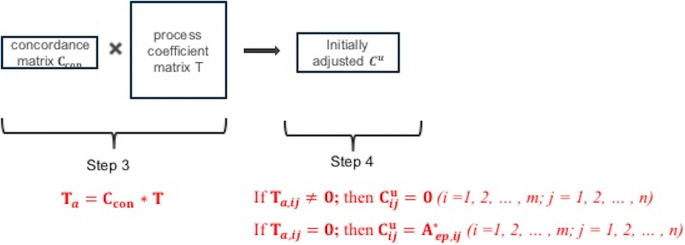

  

  Workflow for preliminary adjustment for double counting

Workflow III: final adjustment of ${\mathbf{C}}^{{\mathbf{u}}}$ for double counting

The steps implemented in workflow II do not avoid double counting completely for several reasons:

• (a) The initially adjusted ${\mathbf{C}}^{{\mathbf{u}}}$ might include inputs from the IO system that are not actually relevant to the specific process of interest because of aggregation. Industries are always an aggregation of heterogeneous processes, and therefore, the technical IO coefficients cannot perfectly represent the production recipe of each individual process belonging to an industry.

• (b) Some processes, which are categorized as “processing” in the process coefficient matrix (e.g., “mowing, by rotary mower,” “milling, aluminum, large parts,” “laminating, foil, with acrylic binder”), are manufacturing sub-processes. These internal sub-processes do not enter the market directly; therefore, upstream inputs should not be allocated to these sub-processes, but only to the final marketable products.

• (c) Process data should already cover all physical material and energy inputs so that equivalent inputs from the IO system would cause double counting (and overestimation of impacts). Due to possible mismatches in concordance and/or aggregation, however, residual inputs from IO material or energy industries may remain in ${\mathbf{C}}^{{\mathbf{u}}}$ after workflow II.

To understand which reason (or reasons in combination) listed above is applicable to each specific process requires detailed expert knowledge and case-by-case investigation. This would be very time-consuming and not universally applicable, and therefore beyond the scope of this study. Two scenarios are adopted to deal with possible cases of double counting and overestimation. Scenario 1 applies moderate double-counting correction (DCC) (${\mathbf{C}}^{{\mathbf{u}}}$_upper in Fig. 3) and leads to upper-boundary results for the hybrid analysis. DCC is more complete in Scenario 2 (${\mathbf{C}}^{{\mathbf{u}}}$_lower in Fig. 3), leading to lower-boundary results. In other words, instead of generating one single hybrid result for each AusLCI process, we generate two sets of hybrid results for each, demonstrating the impact certain assumptions have on the final results.

DCC 1 (${\mathbf{C}}^{{\mathbf{u}}}$_upper):

In response to reasons a) and b) above, it is first assumed that all industries which have processes allocated to in the concordance matrix ${\mathbf{C}}_{{{\mathbf{con}}}}$ should be excluded from contributing to the upstream inputs as process data are generally considered to be product-specific and more reliable than its corresponding, aggregated IO data [Eqs. (9) and (10)]. In addition to workflow II, this removes further upstream IO inputs that should not be used by the corresponding process, thus suppressing the aggregation errors introduced by the corresponding IO industry. Secondly, all sub-processes which do not deliver marketable products directly are internal to the manufacturing processes. Upstream inputs from the IO system are therefore assumed inappropriate and set to zeros for these processes [Eqs. (11) and (12)]. In this study, 462 out of 4463 AusLCI processes are considered as internal manufacturing processes.

$$ {\text{if}}\;\mathop \sum \limits_{{\varvec{i} = 1}}^{\varvec{m}} \mathbf{C}_{{\mathbf{con},\;\mathbf{ ij}}} \varvec{ } \ne 0\;\left( {j = {\mathit{1}}, {\mathit{2}}, \ldots ,n} \right);\;{\text{then}}\;\mathbf{C}_{{\mathbf{ij}}}^{{\mathbf{u}\_\mathbf{upper}}} = 0\;\left( {i = {\mathit{1}}, {\mathit{2}}, \ldots ,m;\quad j = {\mathit{1}}, {\mathit{2}}, \ldots ,n} \right) $$

(9)

$$ {\text{if}}\;\mathop \sum \limits_{{\varvec{i} = 1}}^{\varvec{m}} \mathbf{C}_{{\mathbf{con},\;\mathbf{ ij}}} = 0\;\left( {j = {\mathit{1}}, {\mathit{2}}, \ldots ,n} \right);\;{\text{then}}\;\mathbf{C}_{{\mathbf{ij}}}^{{\mathbf{u}\_\mathbf{upper}}} = \mathbf{A}_{{\mathbf{ep},\mathbf{ ij}}}^{\mathbf{*}} \;\left( {i = {\mathit{1}}, {\mathit{2}}, \ldots ,m;\quad j = {\mathit{1}}, {\mathit{2}}, \ldots ,n} \right) $$

(10)

$$ \begin{aligned} {\text{if}}\;{\mathbf{T}}_{{\mathbf{j}}} \; & (j = {\mathit{1}}, {\mathit{2}}, \ldots ,n)\;{\text{is}}\;{\text{an}}\;{\text{internal}}\;{\text{process}}; \\ & {\text{then}}\;{\mathbf{C}}_{{{\mathbf{ij}}}}^{{{\mathbf{u}}\_{\mathbf{upper}}}} = {\mathbf{0}}\left( {i = {\mathit{1}}, {\mathit{2}}, \ldots ,m;\quad j = {\mathit{1}}, {\mathit{2}}, \ldots ,n} \right) \\ \end{aligned} $$

(11)

$$ \begin{aligned} {\text{if}}\;\mathbf{T}_{\mathbf{j}} \; & (j = {\mathit{1}}, {\mathit{2}}, \ldots ,n)\;{\text{is}}\;{\text{not}}\;{\text{an}}\;{\text{internal}}\;{\text{process}}; \\ & {\text{then}}\;{\mathbf{C}}_{{{\mathbf{ij}}}}^{{{\mathbf{u}}\_{\mathbf{upper}}}} = {\mathbf{A}}_{{{\mathbf{ep}}, {\mathbf{ij}}}}^{*} \;\left( {i = {\mathit{1}}, {\mathit{2}}, \ldots ,m;\quad j = {\mathit{1}}, {\mathit{2}}, \ldots ,n} \right) \\ \end{aligned} $$

(12)

DCC 2 (${\mathbf{C}}^{{\mathbf{u}}}$_lower):

In response to reasons a), b) and c), a third assumption is added, that is, all physical materials and energy inputs are assumed to be covered in the process coefficient matrix already and all material- and energy-related upstream IO inputs are set to zeros [Eqs. (13) and (14)]. This bold assumption holds if the quality of the process coefficient matrix is extremely high and / or the IO table, on average, cannot well represent their corresponding processes. If the process coefficient matrix is with extremely high quality, it is supposed to cover as many physical inputs as possible; and if the IO table is not a good representative, less use of IO inputs would help reduce the possibility of double counting. In our IO system, 1029 industries are about materials manufacturing, construction, transport and energy generation (Additional file 1: Table S1), so we exclude them from the upstream cut-off matrix in this conservative scenario.

$$ {\text{if}}\;{\text{industry}}\;i\;{\text{is}}\;{\text{not}}\;{\text{a}}\;{\text{service}}\;{\text{industry;}}\;{\text{then}}\;\mathbf{C}_{{\mathbf{ij}}}^{{\mathbf{u}\_\mathbf{lower}}} = 0\;\left( {i = {\mathit{1}}, {\mathit{2}}, \ldots ,m;\quad j = 1,2, \ldots ,n} \right) $$

(13)

$$ {\text{if}}\;{\text{industry}}\;i\;{\text{is}}\;{\text{a}}\;{\text{service}}\;{\text{industry;}}\;{\text{then}}\;\mathbf{C}_{{\mathbf{ij}}}^{{\mathbf{u}\_\mathbf{lower}}} = \mathbf{C}_{{\mathbf{ij}}}^{{\mathbf{u}\_\mathbf{upper}}} \;\left( {i = {\mathit{1}}, {\mathit{2}}, \ldots ,m;\quad j = {\mathit{1}}, {\mathit{2}}, \ldots ,n} \right) $$

(14)

2.5 Monte Carlo analysis

Both process-based LCA and EEIOA are associated with various types of assumptions and uncertainties on their own, including parameter and input data uncertainty (e.g., allocation errors, price homogeneity, linearity, aggregation uncertainty, geographical variation, temporal discrepancies), model uncertainty (e.g., impact categories, characterization factors), and scenario uncertainty (e.g., different choices of scope, cut-off criteria) (Peters 2006; Wiedmann 2009; Rowley et al. 2009; Lenzen 2000; Heijungs and Lenzen 2014; Ercan and Tatari 2015; Williams et al. 2009). Specific to the hLCA model developed in this study, two major stochastic uncertainties are investigated further: (1) the unit conversion conducted during the creation of the ${\mathbf{C}}^{{\mathbf{u}}}$ matrix because of price uncertainty (see Sect. 2.4); and (2) the uncertainty associated with adding the EEIO data in the upstream cut-off matrix (Wiedmann et al. 2011; Wolfram et al. 2016; Teh et al. 2017).

Monte Carlo simulation is commonly employed in LCA and EEIOA to quantify the propagation of errors in the model (Peters 2006; Bullard and Sebald 1977; Lenzen 2000). In this study, a Monte Carlo sensitivity analysis for price variation and a Monte Carlo uncertainty analysis for EEIOA data variation are conducted for each DCC scenario to demonstrate the effect on hybrid carbon footprint intensities (CFIs). As for price variation, it is assumed to follow normal distribution with a relative standard deviation (σ) of 30%, which means 99.7% of the prices vary between 10% (1 − 3σ) and 190% (1 + 3σ) of the original prices. Regarding the EEIO data uncertainty, the relative standard deviation for each cell of the SUT and extension matrix has been taken from the routine outputs of MRIO table compilation in the IELab (Lenzen et al. 2014).

3 Results

After creating the upstream cut-off matrix according to Sect. 2.4, the hybrid matrix is completed and presented in Sect. 3.1. Hybrid carbon footprint intensities [CFIs or life-cycle GHG inventories, equivalent to $\mathbf{q}_{\mathbf{h}}$ in Eq. (1)] are then calculated for all AusLCI processes, and the shares of IO inputs are quantified (Sect. 3.2). Upstream IO inputs are further decomposed to show the major contributions from the background economy (Sect. 3.3). Following that, the results of the Monte Carlo simulations are presented in Sect. 3.4.

3.1 Results from different ${\mathbf{C}}^{{\mathbf{u}}}$ double-counting correction scenarios

The effect of workflows II (initial adjustment) and III (upper and lower DCC scenarios) on the ${\mathbf{C}}^{{\mathbf{u}}}$ matrix is visualized in the heatmaps (Fig. 6), showing the absolute size of cell entries. From the initial adjustment to the upper- and lower-bound scenarios, more and more IO upstream inputs are excluded making the upstream cut-off matrix less and less dense.

Fig. 6

Heatmaps of the hybrid matrix, showing how the upstream cut-off matrix C^u is populated under different scenarios for double-counting correction

Following Eq. (1) with ${\tilde{\text{y}}}$ being a column of 1 s, hybrid CFIs of all AusLCI processes are calculated after initial adjustment, upper- and lower-bound DCC, respectively. Out of 4463 hybrid CFIs, 138 are zero, including 32 disposal processes, 17 dummy processes and 89 by-product processes, which have no direct inputs, no direct emissions and no unit prices from the process coefficient matrix. In the following, results for the remaining 4325 processes are presented.

The effect on hybrid CFIs resulting from the different double-counting corrections is significant. As shown in Fig. 7, the upper-bound scenario reduces the average hybrid CFIs across all 4325 processes by 45%, compared to the initial adjustment of C^u. And a further 8% average reduction is caused by adopting lower-bound scenario, indicating the dominating role played by the upper-bound assumption in correcting double counting (and overestimation).

Fig. 7

Reductions of hybrid carbon footprint intensities for 4325 AusLCI processes from initially adjusted scenario to upper-bound scenario and lower-bound scenario, respectively, in relative terms

Closer analysis reveals that the difference between initially adjusted and DCC-corrected hybrid CFIs is largest where corresponding IO industries are highly aggregated. For example, the process “2332 irrigation, pipe irrigation system” is corresponding to the IO industry “5290020 Services to agriculture nec,” but this industry covers not only farm irrigation service, but also other agricultural support services like fruit or vegetable picking, seed grading or cleaning. As a result, the technical IO coefficients of this industry cannot perfectly represent the inputs of the targeted process “pipe irrigation system,” potentially giving rise to overestimation. The upper-bound DCC scenario can effectively treat this type of overestimation by removing this industry from the upstream cut-off matrix. Similar examples are processes that correspond to IO industries like “29000010 Waste collection, treatment disposal remediation and materials recovery services,” “26190010 Electricity generation nec,” “31090010 Non-building construction nec,” “18130090 Other inorganic chemicals nec,”. In contrast, if a process has a more equivalent match with an IO industry, then the differences caused by different DCC scenarios are not that significant. For example, the hybrid CFI of process “1833 general purpose cement, Australian average” is only reduced by 16% when adopting the upper-bound DCC scenario because its corresponding IO industry “20310010 Cement (incl hydraulic and portland)” is a more equivalent representative.

On average, the hybrid CFIs are reduced by 16% when going from the upper- to the lower-bound DCC scenario. (This is different from the 8% mentioned above. The denominator of the 8% is the hybrid CFIs after initial adjustment of C^u, while the denominator of the 16% is the upper-bound hybrid CFIs.) In reverse, the hybrid CFIs are increased by 19% from lower-bound to upper-bound. This means scenarios made for double-counting correction lead to an average variation of (− 16% to + 19%). In addition to the aggregation errors mainly dealt with by the upper-bound DCC scenario, the lower-bound scenario deals with double counting related to physical process inputs. If physical process inputs are complete but the corresponding C^u cells are still filled with irrelevant IO inputs, the lower-bound scenario can help remove these IO inputs, leading to a larger reduction from upper-bound scenario. For instance, process “600 Cottonseed oil, at oil mill” is a complete process that has already covered all physical inputs, but its corresponding IO industry “11500010 Crude soya bean, cotton seed, peanut, sunflower, safflower, rape seed, coconut and vegetable oils” has too many irrelevant inputs which can be effectively removed by the lower-bound scenario. Larger gaps between upper and lower bound also occur if process inputs are incomplete, and the lower-bound DCC incorrectly eliminates necessary inputs from the upstream cut-off matrix so that the resulting hybrid CFIs are underestimated. Take process “86 Aircraft, freight” as an example. In the process coefficient matrix, this process has inputs from “Aluminum’,” “Electricity,” “Light fuel oil,” “Natural gas,” “Polyethylene, HDPE,” “Tap water,” “Transport” and “Treatment, sewage,” but some important inputs are missing, which can be found from its corresponding IO industry “23940010 Aircraft and aircraft parts,” including “Tires, rubber nec,” “Safety glass,” “Iron and steel bars,” “Painted, varnished or coated steel sheet,” “Copper, copper alloy and semi-finished products,” “Radio and radar equipment, navigational aids, and radio remote control equipment” and “dry cell battery.” These missing inputs are incorrectly deleted by the lower-bound scenario, enlarging the difference between upper- and lower-bound DCC.

To sum up, the upper-bound scenario may overestimate the hybrid CFIs for complete processes, and the lower-bound scenario may underestimate the hybrid CFIs for incomplete processes. Since evaluating the completeness of every process is practically impossible without investigating every process individually, simply applying the lower-bound scenario for all processes is a better way to treat double counting (and overestimation). Even if this simplified DCC might cause underestimation for certain processes, the resulting hybrid CFIs can be seen as conservative, yet more realistic, estimate than their corresponding process-based CFIs. With that being said, the most robust outcomes of this hybrid analysis apply to processes whose IO counterparts are equivalent representations, because the hybrid CFIs for these processes remain relatively stable, regardless of the scenarios made for DCC.

3.2 Hybrid carbon footprint intensities

Both upper- and lower-bound hybrid CFIs of 4325 AusLCI processes in absolute terms are illustrated in Fig. 8, with process-based CFIs on the abscissa and both hybrid CFIs on the ordinate. All hybrid CFIs are higher than their corresponding process-based CFIs independent of their absolute values which cover a large range from 1.0E−7 to 1.0E+11 kg CO₂e per functional unit (which can be as small as using a computer for one second or as large as building one entire hydropower plant).

Fig. 8

Hybrid (upper- and lower-bound DCC) versus process-based carbon footprint intensities of 4325 AusLCI processes

As expected, the upper-bound DCC scenario has a higher average share of IO inputs (32%), compared to the lower-bound scenario with 21% on average (Fig. 9). This implies that the average truncation error of pure process-based analysis is between 21% and 32%, which is in agreement with previous studies that found truncation errors ranging from 10% (Bullard et al. 1978) to 50% (Lenzen 2008; Crawford 2008). In both scenarios, the share of IO component varies with the type of process and ranges from 0% to 100%. Zero IO shares are associated with some disposal processes whose unit prices are 0 s, and the 100% IO shares are associated with processes whose input entries are nearly empty in the process coefficient matrix. Among 4325 processes, IO shares are larger than 50% for 325 processes (about 8%) under the lower-bound scenario and 913 processes (about 21%) under the upper-bound scenario. The reasons for these high IO shares are: (1) Some processes in the process coefficient matrix have very few input data so that the process-based analysis largely underestimates the CFIs of these processes. For example, process “2226 Aircraft” only has inputs from “Aluminum” and “Reinforcing steel,” and its direct GHG emissions are zero; and/or (2) the unit prices of some products are not applicable to the Australian context leading to biased estimations. For example, changing the price of process “4437 Work at home, corporate access” would significantly alter its hybrid CFI; and/or (3) the concordance between processes and industries is not appropriate for some processes, meaning the IO industry does not represent the corresponding processes well; and/or (4) the quality of some IO data is impaired when generating a SUT with such high resolution as industry disaggregation may be based on proxy information and imputed top down.

Fig. 9

Process share and IO share in each hybrid CFI under upper-bound DCC scenario (top) and lower-bound scenario (bottom). The percentages shown on the left-hand side (LHS) ordinate of each graph are the shares of process components. Deducting each of them from 100% gives the share of IO components. The values on the right-hand side (RHS) ordinate of each graph show the percentages of AusLCI hybrid CFIs whose process shares are located within the deciles of the LHS ordinate (adding up to 100%). For example, under lower-bound DCC, the process shares of 28% AusLCI hybrid CFIs are between 90% and 100%

3.3 Nature of IO contributions to hybrid CFIs

In order to demonstrate where the missing upstream inputs come from, the contributions from the IO system to hybrid CFIs are decomposed further. For easier presentation, the original 1284 IO industries are aggregated into 19 broad industries following ANZSIC06 divisions (ABS 2008).

The decomposition suggests for both scenarios that “Rental, hiring and real estate services,” “Professional, scientific and technical services,” “Financial and insurance services,” “Wholesale trade” and “Administrative and support services” are the major contributing IO industries (Fig. 10). One significant difference between the DCC scenarios is that for the upper-bound scenario the “Manufacturing” sector is the dominating share taking up 34% of the upstream contribution, whereas in the lower-bound scenario, “Manufacturing” only plays a marginal role. This is due to the fact that in the upper-bound scenario, upstream inputs from “manufacturing” industry complement the physical inputs missing in the process coefficient matrix for auxiliary manufacturing processes. Since the lower-bound scenario excludes all materials manufacturing, facilities construction and energy production industries, the contribution from these industries become insignificant, relative to service industries.

Fig. 10

Contributions to upper-bound (top) and lower-bound hybrid CFIs (bottom) from aggregated IO industries, in relative terms. The relative contribution from a broad industry is shown in brackets after its name

3.4 Monte Carlo analysis

A Monte Carlo sensitivity analysis for price variation and a Monte Carlo uncertainty analysis for IO data are conducted for each DCC scenario (Figs. 11, 12). Each simulation has 5000 runs and takes 8–15 h to complete.

Fig. 11

Relative changes of hybrid CFIs against price variations under upper-bound DCC (LHS) and lower-bound DCC (RHS), sorted in descending order. Original hybrid CFIs correspond to 100%. For each AusLCI process, the high variation and low variation of its hybrid CFI are the results of adding and subtracting one relative standard deviation to and from the ratio of mean value to original value, respectively

Fig. 12

Relative uncertainties of hybrid CFIs against SUT data uncertainties under upper-bound DCC (LHS) and lower-bound DCC (RHS), sorted in descending order. Original hybrid CFIs correspond to 100%. For each AusLCI process, the high uncertainty and low uncertainty of its hybrid CFI are the results of adding and subtracting one relative standard deviation to and from the ratio of mean value to original value, respectively

Assuming the unit price of each AusLCI process follows normal distribution with a relative standard deviation of 30%, we find the resulting hybrid CFIs vary from − 31% to + 33% for the upper-bound scenario and ± 31% for the lower-bound scenario. The average variation across 4325 hybrid CFIs is from − 4.7% to + 5.1% for upper-bound DCC and from − 3.3% to + 3.2% for lower-bound DCC. In general, all upper-bound hybrid CFIs have slightly wider ranges than their corresponding lower-bound ones because upper-bound DCC involves more IO inputs, requiring more unit conversions. Larger variations are normally associated with processes having lower ratios of process-based CFI to hybrid CFI. These processes have higher percentages of IO inputs, which makes them more sensitive to price variations.

The Monte Carlo analysis of SUT data shows that, again, all upper-bound hybrid CFIs have slightly higher uncertainties (ranging from − 5% to + 15%) than their corresponding lower-bound ones (ranging from − 2% to + 11%). On average, the upper-bound hybrid CFIs across 4325 processes change between + 1.4% and + 2.4%, and the lower-bound hybrid CFIs change between + 0.7% and + 1.4%. The bias toward higher values is due to the idiosyncrasies of the IO calculus, which involves a matrix inversion, and is well known from the literature (Lenzen 2000; Lenzen et al. 2010).

Again, a correlation between larger uncertainty and lower ratios of process-based CFI to hybrid CFI can be observed. This is also because low ratios mean relative higher IO shares, leading to larger uncertainty attributed to IO data uncertainty. As a consequence, processes with very high hybrid CFIs, relative to their corresponding process-based CFIs, are more uncertain than the ones with relatively lower hybrid CFIs.

4 Discussion and conclusion

4.1 Opportunities and advantages

Although hybrid LCA is developed with the intention to deal with the shortcomings of process-based LCA and EEIOA to enable a specific as well as complete LCA, its practical application is still rather limited. The hLCA framework presented in this study expands the accessibility of hybrid LCA from specialists to LCA practitioners by developing a streamlined and semi-automated hybrid LCA routine that allows for any process database (in matrix form) to be hybridized with IO data and to be read by LCA software in the same way as conventional databases. The workflow routines generate hybridized database independent of the size of either process or IO data, as long as suitable price information and concordance matrix are available.

The routine is demonstrated in the Australian IELab, combining the most detailed Australian SUT with Australian LCI process data, to quantify the hybrid carbon footprint intensities of all processes. It follows the general IELab workflow structure, in which disparate, unaligned and non-harmonized datasets are processed on one platform, matched with suitable concordance matrices and merged into a more comprehensive system that can be used, adapted and automated further for subsequent analyses on the same platform (Lenzen et al. 2014). Neither the quality of source data nor the representativeness of IO data is ideal for all AusLCI processes, which is why results are presented as a range of hybrid CFIs reflecting modeling settings and assumptions on double-counting correction. For each process, these upper- and lower-bound estimates help the practitioner to quickly identify areas if and where further improvements might be necessary. When more suitable data become available for specific applications, the model can be easily refined to produce more precise hybrid results. Even if no further efforts are taken, the hybrid CFIs generated from this study are still more complete and therefore generally more accurate than pure process-based CFIs. This is because, on average across all AusLCI processes:

• the truncation of pure process-based analysis is between 21% (lower-bound scenario) and 32% (upper-bound scenario);

• scenarios on double-counting correction set boundaries for the hybrid system where the upper boundary is 19% higher than the lower boundary and the lower boundary is 16% lower than the upper boundary;

• uncertainty of price variation introduces a stochastic error from − 4.7% to + 5.1% (upper-bound scenario) and from − 3.3% to + 3.2% (lower-bound scenario);

• uncertainty of IO data introduces a stochastic error between + 1.4% and + 2.4% (upper-bound scenario) and between + 0.7% and + 1.4% (lower-bound scenario).

These results clearly suggest that truncation is a more significant source of (systematic) error than either price variation, IO data uncertainty or scenarios on how the upstream cut-off matrix is populated.

Which hybrid result to take for further applications depends on the quality of source data (i.e., IO data, process data, price data and the concordance matrix) as well as the representativeness of the IO data. Higher quality of source data and more equivalent representation of IO data would generally suggest the upper side of the hybrid results, while lower quality of source data and less equivalent representation of IO data would suggest lower-bound results which also constitute a more conservative, i.e., cautious estimate. In this study, for 91% of the modeled processes, the upper bound and lower bound of each process lies between + /− 20% of the average hybrid CFI, respectively, and the mean average value is recommended.

Although the data employed in our work are Australian specific, the underlying procedure can be applied to any country or region with available IO tables. The benefit for decision-makers and LCA practitioners lies in the fact that upstream sources of environmental impacts are automatically included, which are usually neglected in conventional LCA studies (Lake et al. 2015; Kjaer et al. 2015).

It should also be noted that the hybrid LCA routine is flexible in the way that once specific process flows to the background economy become necessary for a specific research question, the downstream cut-off matrix ${\mathbf{C}}^{{\mathbf{d}}}$ can be efficiently added to this routine to accomplish a fully integrated hLCA.

4.2 Limitations and challenges

In spite of the advances made here, several limitations and challenges remain in implementing this hLCA model. As demonstrated above, the most significant impact on the results stems from correcting for double counting when creating the ${\mathbf{C}}^{{\mathbf{u}}}$ matrix. Several approaches have been described previously to deal with double counting, including Leontief’s price model (Strømman and Solli 2008), adjustments based on structural path analysis (Strømman et al. 2009) and system incompleteness factors (Rowley et al. 2009). However, none of them have been applied to multiple processes simultaneously due to the nature of the method and/or the complexity of the algorithms. To enable hybrid analysis at the database level, a more generalized method is adopted in this study, but admittedly, the accurate removal of double counting cannot be guaranteed because the actual data employed are not ideal.

First and foremost, the availability of price data is one of major concerns when constructing the upstream cut-off matrix. Since finding accurate price data of all Australian processes is unrealistically time-consuming, ecoinvent price information is used instead which reflects a different economy and can only be seen as an estimate. Even though we find a low sensitivity to prices from the Monte Carlo simulation, country-, sector- and year-specific price databases would certainly increase accuracy.

The second major concern is related to the concordance matrix between process and IO industries. Although the most detailed SUT available is used, correctly matching processes with industries is potentially prone to inconsistencies and mistakes. There are cases where heterogeneous processes have to be matched with one single broad industry (e.g., both “disposal of plastic” and “waste treatment, textiles” are allocated to “waste collection, treatment disposal remediation and materials recovery services”) or one single process might be matched to multiple industries (e.g., “transport, passenger car” can belong to both “urban road passenger transport services” and “interurban road passenger transport services”).

Thirdly, the temporal dimension is not consistent between the process and IO systems. The process system covers multiple years and could potentially be matched to IO systems from different years. However, this would be substantially more difficult to implement, and in this work, IO data for one year only are used (2008/09), because this is the base year in IELab which produces the most reliable IO table. For industries with more advanced technology, matching data years will be more important than for established technologies.

Lastly, the discrepancy of elementary flows between two systems confines the studies to a certain number of indicators. Given the process system has thousands of elementary flows, considerable amount of effort is needed to deliver a comparable elementary flow database for the IO system to enable more comprehensive environmental studies.

4.3 Outlook and further research

As suggested by Suh (2004) and Hertwich et al. (2018), detailed data collection and documentation has always been highly requested for LCA studies. For hybrid LCA, in particular, the prices and sales of products, specific description of input–output industries and wide coverage of environmental extensions for IO tables all play crucial roles. As individual process database and IO table continue to grow and improve, more automated, streamlined and validated ways of compiling hybrid life cycle inventories become more important to produce quality assessments (Crawford et al. 2017). The framework presented in this paper is a step in that direction. Further development of this model can take advantage of highly disaggregated, multi-scale, multi-unit and/or continuously updated input–output tables to create a regionalized and temporally differentiated hybrid LCI database with multiple environmental indicators. The trend to regionalization in LCA is being followed in the IOA community with the creation of more sub-national multi-region input–output databases (Wiedmann and Lenzen 2018), but no efforts have been made yet to create regionalized hybrid datasets.

References

ABS (2008) 1292.0.55.005—Australian and New Zealand Standard Industrial Classification (ANZIC) 2006 Correspondence Tables, Table 5 Correspondences ISIC Rev 4—ANZIC 2006. Australian Bureau of Statistics
ABS (2010) Producer Price Indexes, Australia, Dec 2009. ABS Catalogue Number 6247.0. http://www.abs.gov.au/AUSSTATS/abs@.nsf/allprimarymainfeatures/3273FC7113E0CBD9CA25770E0019138E?opendocument. Accessed 01 Oct 2016
ABS (2012) Australian National Accounts: Input–Output Tables (Product Details)—Electronic Publication, 2008-09. ABS Catalogue Number 5215.0.55.001. http://www.abs.gov.au/AUSSTATS/abs@.nsf/allprimarymainfeatures/116C97E206DE3464CA257C310015E231?opendocument. Accessed 08 Sept 2016
Acquaye AA, Wiedmann T, Feng K, Crawford RH, Barrett J, Kuylenstierna J, Duffy AP, Koh SC, McQueen-Mason S (2011a) Identification of ‘carbon hot-spots’ and quantification of GHG intensities in the biodiesel supply chain using hybrid LCA and structural path analysis. Environ Sci Technol 45(6):2471–2478
Acquaye AA, Wiedmann T, Kuishang F, Crawford RH, Barrett J, Kuylenstierna J, Duffy AP, Koh SCL, McQueen-Mason S (2011b) Identification of ‘carbon hot-spots’ and quantification of GHG intensities in the biodiesel supply chain using hybrid LCA and structural path analysis. Environ Sci Technol 45(6):2471–2478
AGEIS (2016) Australian Greenhouse Emissions Information System. http://www.environment.gov.au/climate-change/climate-science-data/greenhouse-gas-measurement/ageis. Accessed 15 Sept 2016
Baboulet O, Lenzen M (2010) Evaluating the environmental performance of a university. J Clean Prod 18(12):1134–1141
Bullard CW, Sebald AV (1977) Effects of parametric uncertainty and technological change on input–output models. Rev Econ Stat 59(1):75–81
Bullard CW, Penner PS, Pilati DA (1978) Net energy analysis—handbook for combining process and input–output analysis. Res Energy 1(3):267–313
Bush R, Jacques DA, Scott K, Barrett J (2014) The carbon payback of micro-generation: an integrated hybrid input–output approach. Appl Energy 119:85–98
Changbo W, Lixiao Z, Shuying Y, Mingyue P (2012) A hybrid life-cycle assessment of nonrenewable energy and greenhouse-gas emissions of a village-level biomass gasification project in China. Energies 5(8):2708–2723
Crawford RH (2008) Validation of a hybrid life-cycle inventory analysis method. J Environ Manage 88(3):496–506
Crawford RH, Bontinck P-A, Stephan A, Wiedmann T (2017) Towards an automated approach for compiling hybrid life cycle inventories. Proc Eng 180(Supplement C):157–166
Crawford RH, Bontinck P-A, Stephan A, Wiedmann T, Yu M (2018) Hybrid life cycle inventory methods—a review. J Clean Prod 172(SupplementC):1273–1288
Dadhich P, Genovese A, Kumar N, Acquaye AA (2015) Developing sustainable supply chains in the UK construction industry: a case study. Int J Prod Econ 164:271–284
Ercan T, Tatari O (2015) A hybrid life cycle assessment of public transportation buses with alternative fuel options. Int J Life Cycle Assess 20(9):1213–1231
Eurostat (2008) Eurostat manual of supply, use and input–output tables. Office for Official Publications of the European Communities, Luxembourg
Feng K, Hubacek K, Siu YL, Li X (2014) The energy and water nexus in Chinese electricity production: a hybrid life cycle analysis. Renew Sustain Energy Rev 39:342–355
Ferrão P, Nhambiu J (2009) A comparison between conventional LCA and hybrid EIO-LCA: analyzing crystal giftware contribution to global warming potential. In: Suh S (ed) Handbook of input–output economics in industrial ecology. Springer, Dordrecht
Frischknecht R, Jungbluth N, Althaus H-J, Doka G, Dones R, Heck T, Hellweg S, Hischier R, Nemecek T, Rebitzer G, Spielmann M (2005) The ecoinvent database: overview and methodological framework. Int J Life Cycle Assess 10(1):3–9
Geschke A (2017) Balancing datafeed. Industrial Ecology Virtual Laboratory (Australian IELab). https://ielab.info, https://ielab-aus.info. Sept 2017
Geschke A, Hadjikakou M (2017) Virtual laboratories and MRIO analysis—an introduction. Econ Syst Res 29(2):143–157
Gibon T, Schaubroeck T (2017) Lifting the fog on characteristics and limitations of hybrid LCA—a reply to “Does hybrid LCA with a complete system boundary yield adequate results for product promotion?” by Yang Y (Int J Life Cycle Assess) 22(3):456–406. https://doi.org/10.1007/s11367-016-1256-9. Int J Life Cycle Assess 22(6):1005–1008
Grant T (2015) AusLCI Database Manual v1.1. Australian Life Cycle Assessment Society (ALCAS)
Heijungs R, Lenzen M (2014) Error propagation methods for LCA—a comparison. Int J Life Cycle Assess 19(7):1445–1461
Heijungs R, Suh S (2002) The computational structure of life cycle assessment. In: Tukker A (ed) Eco-efficiency in industry and science. Springer, Dordrecht, vol 11
Hertwich E, Heeren N, Kuczenski B, Majeau-Bettez G, Myers RJ, Pauliuk S, Stadler K, Lifset R (2018) Nullius in verba: advancing data transparency in industrial ecology. J Ind Ecol
Inaba R, Nansai K, Fujii M, Hashimoto S (2010) Hybrid life-cycle assessment (LCA) of CO2 emission with management alternatives for household food wastes in Japan. Waste Manage Res 28(6):496–507
Junnila SI (2006) Empirical comparison of process and economic input–output life cycle assessment in service industries. Environ Sci Technol 40(22):7070–7076
Kjaer LL, Høst-Madsen NK, Schmidt JH, McAloone TC (2015) Application of environmental input–output analysis for corporate and product environmental footprints-learnings from three cases. Sustainability 7(9):11438–11461
Lake A, Acquaye A, Genovese A, Kumar N, Koh SCL (2015) An application of hybrid life cycle assessment as a decision support framework for green supply chains. Int J Prod Res 53(21):6495–6521
Lane J (2017) Greenhouse gas datafeed. Industrial ecology virtual laboratory (Australian IELab), https://ielab.info, https://ielab-aus.info. Sept 2017
Lenzen M (2000) Errors in conventional and input–output-based life-cycle inventories. J Ind Ecol 4(4):127–148
Lenzen M (2008) Errors in conventional and input–output—based life—cycle inventories. J Ind Ecol 4(4):127–148
Lenzen M (2017) Initial estimate datafeed. Industrial Ecology Virtual Laboratory (Australian IELab), https://ielab.info, https://ielab-aus.info. Sept 2017
Lenzen M, Crawford RH (2009) The path exchange method for hybrid LCA. Environ Sci Technol 43(21):8251–8256
Lenzen M, Wood R, Wiedmann T (2010) Uncertainty analysis for multi-region input–output models—a case study of the UK’s carbon footprint. Econ Syst Res 22(1):43–63
Lenzen M, Geschke A, Wiedmann T, Lane J, Anderson N, Baynes T, Boland J, Daniels P, Dey C, Fry J, Hadjikakou M, Kenway S, Malik A, Moran D, Murray J, Nettleton S, Poruschi L, Reynolds C, Rowley H, Ugon J, Webb D, West J (2014) Compiling and using input–output frameworks through collaborative virtual laboratories. Sci Total Environ 485–486:241–251
Lenzen M, Geschke A, Malik A, Fry J, Lane J, Wiedmann T, Kenway S, Hoang K, Cadogan-Cowper A (2017) New multi-regional input–output databases for Australia—enabling timely and flexible regional analysis. Econ Syst Res 29(2):275–295
Majeau-Bettez G, Strømman AH, Hertwich EG (2011) Evaluation of process- and input–output-based life cycle inventory data with regard to truncation and aggregation issues. Environ Sci Technol 45(23):10170–10177
Majeau-Bettez G, Wood R, Stromman AH (2014) Unified theory of allocations and constructs in life cycle assessment and input–output analysis. J Ind Ecol 5:747
Malik A, Lenzen M, Ralph PJ, Tamburic B (2015) Hybrid life-cycle assessment of algal biofuel production. Biores Technol 184:436–443
Malik A, Lenzen M, Geschke A (2016) Triple bottom line study of a lignocellulosic biofuel industry. GCB Bioener 8:96–110
Miller RE, Blair PD (2009) Input–output analysis : foundations and extensions, 2nd edn. Cambridge University Press, Cambridge
Nakamura S, Nansai K (2016) Input–output and hybrid LCA. In: Finkbeiner M (ed) Special types of life cycle assessment. Springer, Dordrecht
OFX (2017) Historical exchange rates. https://www.ofx.com/en-au/forex-news/historical-exchange-rates/. Accessed 16 Feb 2017
Peters GP (2006) Efficient algorithms for life cycle assessment, input–output analysis, and Monte-Carlo analysis. Int J Life Cycle Assess 12(6):373
Peters GP (2010) Carbon footprints and embodied carbon at multiple scales. Curr Opin Environ Sustain 2:245–250
Peters GP, Hertwich EG (2006) A comment on “Functions, commodities and environmental impacts in an ecological-economic model”. Ecol Econ 59(1):1–6
Pomponi F, Lenzen M (2018) Hybrid life cycle assessment (LCA) will likely yield more accurate results than process-based LCA. J Clean Prod 176:210–215
Rowley HV, Lundie S, Peters GM (2009) A hybrid life cycle assessment model for comparison with conventional methodologies in Australia. Int J Life Cycle Assess 14(6):508–516
Schaubroeck T, Gibon T (2017) Outlining reasons to apply hybrid LCA—a reply to “rethinking system boundary in LCA” by Yi Yang (2017). Int J Life Cycle Assess 22(6):1012–1013
Stephan A, Crawford RH, Bontinck P (2018) A model for streamlining and automating path exchange hybrid life cycle assessment. Int J Life Cycle Assess
Strømman AH, Solli C (2008) Applying Leontief’s price model to estimate missing elements in hybrid life cycle inventories. J Ind Ecol 12(1):26–33
Strømman AH, Peters GP, Hertwich EG (2009) Approaches to correct for double counting in tiered hybrid life cycle inventories. J Clean Prod 17:248–254
Suh S (2004) Functions, commodities and environmental impacts in an ecological-economic model. Ecol Econ 48(4):451–467
Suh S (2006) Reply: downstream cut-offs in integrated hybrid life-cycle assessment. Ecol Econ 59(1):7–12
Suh S, Huppes G (2000) Gearing input–output model to LCA, part I: general framework for hybrid approach. CML, Leiden University, Leiden
Suh S, Huppes G (2005) Methods for Life Cycle Inventory of a Product. J Clean Prod 13:687–697
Suh S, Lippiatt BC (2012) Framework for hybrid life cycle inventory databases: a case study on the Building for Environmental and Economic Sustainability (BEES) database. Int J Life Cycle Assess 5:604
Suh S, Lenzen M, Treloar GJ, Hondo H, Horvath A, Huppes G, Jolliet O, Klann U, Krewitt W, Moriguchi Y, Munksgaard J, Norris G (2004) System boundary selection in life-cycle inventories using hybrid approaches. Environ Sci Technol 38(3):657–664
Teh SH, Wiedmann T, Castel A, de Burgh J (2017) Hybrid life cycle assessment of greenhouse gas emissions from cement, concrete and geopolymer concrete in Australia. J Clean Prod 152(Supplement C):312–320
Teh SH, Wiedmann T, Moore S (2018) Mixed-unit hybrid life cycle assessment applied to the recycling of construction materials. J Econ Struct 7(13)
Ward H, Wenz L, Steckel JC, Minx JC (2018) Truncation error estimates in process life cycle assessment using input–output analysis. J Ind Ecol 22:1080–1091
Weidema BP, Bauer C, Hischier R, Mutel C, Nemecek T, Reinhard J, Vadenbo CO, Wernet G (2013) The ecoinvent database: overview and methodology, Data quality guideline for the ecoinvent database version 3
Wiedmann T (2009) A review of recent multi-region input–output models used for consumption-based emission and resource accounting. Ecol Econ 69(2):211–222
Wiedmann T (2017) An input–output virtual laboratory in practice—survey of uptake, usage and applications of the first operational IELab. Econ Syst Res 29(2):296–312
Wiedmann T, Lenzen M (2018) Environmental and social footprints of international trade. Nat Geosci 11:314–321
Wiedmann TO, Suh S, Feng K, Lenzen M, Acquaye AA, Scott K, Barrett JR (2011) Application of hybrid life cycle approaches to emerging energy technologies—the case of wind power in the UK. Environ Sci Technol 45(13):5900–5907
Williams ED, Weber CL, Hawkins TR (2009) Hybrid framework for managing uncertainty in life cycle inventories. J Ind Ecol 13(6):928–944
Wolfram P, Wiedmann T, Diesendorf M (2016) Carbon footprint scenarios for renewable electricity in Australia. J Clean Prod 124:236–245
Yang Y (2016) Does hybrid LCA with a complete system boundary yield adequate results for product promotion? Int J Life Cycle Assess 22(3):456–460
Yang Y (2017) Rethinking system boundary in LCA—reply to “Lifting the fog on the characteristics and limitations of hybrid LCA” by Thomas Gibon and Thomas Schaubroeck (2017). Int J Life Cycle Assess 22(6):1009–1011
Yang Y, Heijungs R, Brandão M (2017) Hybrid life cycle assessment (LCA) does not necessarily yield more accurate results than process-based LCA. J Clean Prod 150:237–242
Zhai P, Williams ED (2010) Dynamic hybrid life cycle assessment of energy and carbon of multicrystalline silicon photovoltaic systems. Environ Sci Technol 44(20):7950–7955
Authors’ contribution
All authors contributed to the research, analysis and manuscript. Both authors read and approved the final manuscript.
Acknowledgements
This research is funded by the Australian Research Council under the Discovery Project DP150100962. The IELab is supported by the Australian Research Council, Grant Number LE160100066. The authors would like to thank Paul-Antoine Bontinck from The University of Melbourne for his help in the construction of the process coefficient matrix and the preliminary concordance matrix (Additional file 1: Figure S1). The authors are grateful to Dr. Majeau‐Bettez Guillaume for his discussions regarding the hybrid LCA model.
Competing interests
The authors declare that they have no competing interests. Author Thomas Wiedmann is also an Editor of the Journal of Economic Structures.
Availability of data and materials